numpy.random.standard_cauchy

random.standard_cauchy(size=None)

從標準柯西分佈（眾數 = 0）中抽取樣本。

也稱為勞倫茲分佈。

注意

新程式碼應使用 standard_cauchy 方法，此方法屬於 Generator 實例；請參閱快速入門。

參數:

sizeint 或 int 元組，選填

輸出形狀。如果給定的形狀是，例如 (m, n, k)，則會抽取 m * n * k 個樣本。預設值為 None，在這種情況下會傳回單一值。

返回:

samplesndarray 或純量

抽取的樣本。

參見

random.Generator.standard_cauchy

新程式碼應使用的方法。

註解

完整柯西分佈的機率密度函數為

\[P(x; x_0, \gamma) = \frac{1}{\pi \gamma \bigl[ 1+ (\frac{x-x_0}{\gamma})^2 \bigr] }\]

標準柯西分佈僅設定 \(x_0=0\) 和 \(\gamma=1\)

柯西分佈出現在驅動諧波振盪器問題的解中，也描述了光譜線展寬。它也描述了以隨機角度傾斜的線切割 x 軸的值分佈。

當研究假設檢定（假設常態性）時，觀察檢定在來自柯西分佈的資料上的表現，是衡量它們對重尾分佈敏感度的好指標，因為柯西分佈看起來很像高斯分佈，但具有更重的尾部。

參考文獻

[1]

NIST/SEMATECH 電子手冊統計方法，「柯西分佈」，https://www.itl.nist.gov/div898/handbook/eda/section3/eda3663.htm

[2]

Weisstein, Eric W. 「柯西分佈。」來自 MathWorld–Wolfram 網路資源。https://mathworld.wolfram.com/CauchyDistribution.html

[3]

維基百科，「柯西分佈」 https://en.wikipedia.org/wiki/Cauchy_distribution

範例

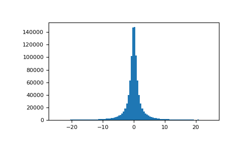
繪製樣本並繪製分佈圖

>>> import matplotlib.pyplot as plt
>>> s = np.random.standard_cauchy(1000000)
>>> s = s[(s>-25) & (s<25)]  # truncate distribution so it plots well
>>> plt.hist(s, bins=100)
>>> plt.show()