

NumPy 快速入門#
先決條件#
您需要具備一些 Python 知識。若要複習,請參閱Python 教學。
若要執行範例,除了 NumPy 之外,您還需要安裝 matplotlib。
學習者概況
這是 NumPy 中陣列的快速概覽。它示範了 n 維 (n\(n>=2\)) 陣列如何表示和操作。特別是,如果您不知道如何將常用函數應用於 n 維陣列(不使用 for 迴圈),或者您想了解 n 維陣列的軸和形狀屬性,本文可能會對您有所幫助。
學習目標
閱讀後,您應該能夠
理解 NumPy 中一維、二維和 n 維陣列之間的差異;
理解如何在不使用 for 迴圈的情況下,將一些線性代數運算應用於 n 維陣列;
理解 n 維陣列的軸和形狀屬性。
基礎知識#
NumPy 的主要物件是同質多維陣列。它是一個元素表格(通常是數字),所有元素都是相同的類型,並由非負整數元組索引。在 NumPy 中,維度稱為軸。
例如,3D 空間中點座標的陣列 [1, 2, 1] 只有一個軸。該軸有 3 個元素,因此我們說它的長度為 3。在下圖的範例中,陣列有 2 個軸。第一個軸的長度為 2,第二個軸的長度為 3。
[[1., 0., 0.],
 [0., 1., 2.]]
NumPy 的陣列類別稱為 ndarray。它也以別名 array 聞名。請注意,numpy.array 與標準 Python 函式庫類別 array.array 不同,後者僅處理一維陣列,功能也較少。ndarray 物件更重要的屬性如下
- ndarray.ndim
陣列的軸(維度)數量。
- ndarray.shape
陣列的維度。這是一個整數元組,表示陣列在每個維度中的大小。對於具有 n 列和 m 行的矩陣,
shape將為(n,m)。shape元組的長度因此是軸的數量,ndim。- ndarray.size
陣列的元素總數。這等於
shape元素的乘積。- ndarray.dtype
描述陣列中元素類型的物件。可以使用標準 Python 類型建立或指定 dtype。此外,NumPy 也提供自己的類型。numpy.int32、numpy.int16 和 numpy.float64 是一些範例。
- ndarray.itemsize
陣列中每個元素的大小(以位元組為單位)。例如,
float64類型元素的陣列具有itemsize8 (=64/8),而complex32類型元素的陣列具有itemsize4 (=32/8)。它等同於ndarray.dtype.itemsize。- ndarray.data
包含陣列實際元素的緩衝區。通常,我們不需要使用此屬性,因為我們將使用索引功能存取陣列中的元素。
範例#
>>> import numpy as np
>>> a = np.arange(15).reshape(3, 5)
>>> a
array([[ 0,  1,  2,  3,  4],
       [ 5,  6,  7,  8,  9],
       [10, 11, 12, 13, 14]])
>>> a.shape
(3, 5)
>>> a.ndim
2
>>> a.dtype.name
'int64'
>>> a.itemsize
8
>>> a.size
15
>>> type(a)
<class 'numpy.ndarray'>
>>> b = np.array([6, 7, 8])
>>> b
array([6, 7, 8])
>>> type(b)
<class 'numpy.ndarray'>
陣列建立#
有多種方法可以建立陣列。
例如,您可以使用 array 函數從常規 Python 列表或元組建立陣列。結果陣列的類型是從序列中元素的類型推導出來的。
>>> import numpy as np
>>> a = np.array([2, 3, 4])
>>> a
array([2, 3, 4])
>>> a.dtype
dtype('int64')
>>> b = np.array([1.2, 3.5, 5.1])
>>> b.dtype
dtype('float64')
常見的錯誤是使用多個引數呼叫 array,而不是提供單個序列作為引數。
>>> a = np.array(1, 2, 3, 4)    # WRONG
Traceback (most recent call last):
  ...
TypeError: array() takes from 1 to 2 positional arguments but 4 were given
>>> a = np.array([1, 2, 3, 4])  # RIGHT
array 將序列的序列轉換為二維陣列,將序列的序列的序列轉換為三維陣列,依此類推。
>>> b = np.array([(1.5, 2, 3), (4, 5, 6)])
>>> b
array([[1.5, 2. , 3. ],
       [4. , 5. , 6. ]])
陣列的類型也可以在建立時明確指定
>>> c = np.array([[1, 2], [3, 4]], dtype=complex)
>>> c
array([[1.+0.j, 2.+0.j],
       [3.+0.j, 4.+0.j]])
通常,陣列的元素最初是未知的,但其大小是已知的。因此,NumPy 提供了幾個函數來建立具有初始佔位符內容的陣列。這些函數最大限度地減少了擴展陣列的必要性,而擴展陣列是一個昂貴的操作。
函數 zeros 建立一個充滿零的陣列,函數 ones 建立一個充滿一的陣列,而函數 empty 建立一個初始內容是隨機的,並且取決於記憶體狀態的陣列。預設情況下,建立的陣列的 dtype 為 float64,但可以透過關鍵字引數 dtype 指定。
>>> np.zeros((3, 4))
array([[0., 0., 0., 0.],
       [0., 0., 0., 0.],
       [0., 0., 0., 0.]])
>>> np.ones((2, 3, 4), dtype=np.int16)
array([[[1, 1, 1, 1],
        [1, 1, 1, 1],
        [1, 1, 1, 1]],

       [[1, 1, 1, 1],
        [1, 1, 1, 1],
        [1, 1, 1, 1]]], dtype=int16)
>>> np.empty((2, 3))
array([[3.73603959e-262, 6.02658058e-154, 6.55490914e-260],  # may vary
       [5.30498948e-313, 3.14673309e-307, 1.00000000e+000]])
若要建立數字序列,NumPy 提供了 arange 函數,它類似於 Python 內建的 range,但會傳回一個陣列。
>>> np.arange(10, 30, 5)
array([10, 15, 20, 25])
>>> np.arange(0, 2, 0.3)  # it accepts float arguments
array([0. , 0.3, 0.6, 0.9, 1.2, 1.5, 1.8])
當 arange 與浮點引數一起使用時,由於有限的浮點精度,通常無法預測獲得的元素數量。因此,通常最好使用 linspace 函數,該函數接收我們想要的元素數量作為引數,而不是步長
>>> from numpy import pi
>>> np.linspace(0, 2, 9)                   # 9 numbers from 0 to 2
array([0.  , 0.25, 0.5 , 0.75, 1.  , 1.25, 1.5 , 1.75, 2.  ])
>>> x = np.linspace(0, 2 * pi, 100)        # useful to evaluate function at lots of points
>>> f = np.sin(x)
列印陣列#
當您列印陣列時,NumPy 會以類似於巢狀列表的方式顯示它,但具有以下佈局
最後一個軸從左到右列印,
倒數第二個軸從上到下列印,
其餘的軸也從上到下列印,每個切片之間用一個空行分隔。
然後,一維陣列列印為行,二維陣列列印為矩陣,三維陣列列印為矩陣列表。
>>> a = np.arange(6)                    # 1d array
>>> print(a)
[0 1 2 3 4 5]
>>>
>>> b = np.arange(12).reshape(4, 3)     # 2d array
>>> print(b)
[[ 0  1  2]
 [ 3  4  5]
 [ 6  7  8]
 [ 9 10 11]]
>>>
>>> c = np.arange(24).reshape(2, 3, 4)  # 3d array
>>> print(c)
[[[ 0  1  2  3]
  [ 4  5  6  7]
  [ 8  9 10 11]]

 [[12 13 14 15]
  [16 17 18 19]
  [20 21 22 23]]]
請參閱下方以取得關於 reshape 的更多詳細資訊。
如果陣列太大而無法列印,NumPy 會自動跳過陣列的中心部分,僅列印角
>>> print(np.arange(10000))
[   0    1    2 ... 9997 9998 9999]
>>>
>>> print(np.arange(10000).reshape(100, 100))
[[   0    1    2 ...   97   98   99]
 [ 100  101  102 ...  197  198  199]
 [ 200  201  202 ...  297  298  299]
 ...
 [9700 9701 9702 ... 9797 9798 9799]
 [9800 9801 9802 ... 9897 9898 9899]
 [9900 9901 9902 ... 9997 9998 9999]]
若要停用此行為並強制 NumPy 列印整個陣列,您可以使用 set_printoptions 變更列印選項。
>>> np.set_printoptions(threshold=sys.maxsize) # sys module should be imported
基本運算#
陣列上的算術運算子會逐元素應用。將建立一個新陣列並填入結果。
>>> a = np.array([20, 30, 40, 50])
>>> b = np.arange(4)
>>> b
array([0, 1, 2, 3])
>>> c = a - b
>>> c
array([20, 29, 38, 47])
>>> b**2
array([0, 1, 4, 9])
>>> 10 * np.sin(a)
array([ 9.12945251, -9.88031624,  7.4511316 , -2.62374854])
>>> a < 35
array([ True,  True, False, False])
與許多矩陣語言不同,乘積運算子 * 在 NumPy 陣列中逐元素運算。矩陣乘積可以使用 @ 運算子(在 python >=3.5 中)或 dot 函數或方法執行
>>> A = np.array([[1, 1],
...               [0, 1]])
>>> B = np.array([[2, 0],
...               [3, 4]])
>>> A * B     # elementwise product
array([[2, 0],
       [0, 4]])
>>> A @ B     # matrix product
array([[5, 4],
       [3, 4]])
>>> A.dot(B)  # another matrix product
array([[5, 4],
       [3, 4]])
某些運算,例如 += 和 *=,會就地執行以修改現有陣列,而不是建立新陣列。
>>> rg = np.random.default_rng(1)  # create instance of default random number generator
>>> a = np.ones((2, 3), dtype=int)
>>> b = rg.random((2, 3))
>>> a *= 3
>>> a
array([[3, 3, 3],
       [3, 3, 3]])
>>> b += a
>>> b
array([[3.51182162, 3.9504637 , 3.14415961],
       [3.94864945, 3.31183145, 3.42332645]])
>>> a += b  # b is not automatically converted to integer type
Traceback (most recent call last):
    ...
numpy._core._exceptions._UFuncOutputCastingError: Cannot cast ufunc 'add' output from dtype('float64') to dtype('int64') with casting rule 'same_kind'
當使用不同類型的陣列運算時,結果陣列的類型對應於更通用或更精確的類型(一種稱為向上轉型的行為)。
>>> a = np.ones(3, dtype=np.int32)
>>> b = np.linspace(0, pi, 3)
>>> b.dtype.name
'float64'
>>> c = a + b
>>> c
array([1.        , 2.57079633, 4.14159265])
>>> c.dtype.name
'float64'
>>> d = np.exp(c * 1j)
>>> d
array([ 0.54030231+0.84147098j, -0.84147098+0.54030231j,
       -0.54030231-0.84147098j])
>>> d.dtype.name
'complex128'
許多一元運算,例如計算陣列中所有元素的總和,都實作為 ndarray 類別的方法。
>>> a = rg.random((2, 3))
>>> a
array([[0.82770259, 0.40919914, 0.54959369],
       [0.02755911, 0.75351311, 0.53814331]])
>>> a.sum()
3.1057109529998157
>>> a.min()
0.027559113243068367
>>> a.max()
0.8277025938204418
預設情況下,這些運算會應用於陣列,就好像它是一個數字列表一樣,而與其形狀無關。但是,透過指定 axis 參數,您可以沿著陣列的指定軸應用運算
>>> b = np.arange(12).reshape(3, 4)
>>> b
array([[ 0,  1,  2,  3],
       [ 4,  5,  6,  7],
       [ 8,  9, 10, 11]])
>>>
>>> b.sum(axis=0)     # sum of each column
array([12, 15, 18, 21])
>>>
>>> b.min(axis=1)     # min of each row
array([0, 4, 8])
>>>
>>> b.cumsum(axis=1)  # cumulative sum along each row
array([[ 0,  1,  3,  6],
       [ 4,  9, 15, 22],
       [ 8, 17, 27, 38]])
通用函數#
NumPy 提供了常見的數學函數,例如 sin、cos 和 exp。在 NumPy 中,這些稱為「通用函數」( ufunc )。在 NumPy 中,這些函數逐元素地對陣列進行運算,並產生一個陣列作為輸出。
>>> B = np.arange(3)
>>> B
array([0, 1, 2])
>>> np.exp(B)
array([1.        , 2.71828183, 7.3890561 ])
>>> np.sqrt(B)
array([0.        , 1.        , 1.41421356])
>>> C = np.array([2., -1., 4.])
>>> np.add(B, C)
array([2., 0., 6.])
索引、切片和迭代#
一維陣列可以像 列表 和其他 Python 序列一樣進行索引、切片和迭代。
>>> a = np.arange(10)**3
>>> a
array([  0,   1,   8,  27,  64, 125, 216, 343, 512, 729])
>>> a[2]
8
>>> a[2:5]
array([ 8, 27, 64])
>>> # equivalent to a[0:6:2] = 1000;
>>> # from start to position 6, exclusive, set every 2nd element to 1000
>>> a[:6:2] = 1000
>>> a
array([1000,    1, 1000,   27, 1000,  125,  216,  343,  512,  729])
>>> a[::-1]  # reversed a
array([ 729,  512,  343,  216,  125, 1000,   27, 1000,    1, 1000])
>>> for i in a:
...     print(i**(1 / 3.))
...
9.999999999999998  # may vary
1.0
9.999999999999998
3.0
9.999999999999998
4.999999999999999
5.999999999999999
6.999999999999999
7.999999999999999
8.999999999999998
多維陣列的每個軸可以有一個索引。這些索引在一個以逗號分隔的元組中給出
>>> def f(x, y):
...     return 10 * x + y
...
>>> b = np.fromfunction(f, (5, 4), dtype=int)
>>> b
array([[ 0,  1,  2,  3],
       [10, 11, 12, 13],
       [20, 21, 22, 23],
       [30, 31, 32, 33],
       [40, 41, 42, 43]])
>>> b[2, 3]
23
>>> b[0:5, 1]  # each row in the second column of b
array([ 1, 11, 21, 31, 41])
>>> b[:, 1]    # equivalent to the previous example
array([ 1, 11, 21, 31, 41])
>>> b[1:3, :]  # each column in the second and third row of b
array([[10, 11, 12, 13],
       [20, 21, 22, 23]])
當提供的索引少於軸的數量時,缺少的索引被視為完整的切片 :
>>> b[-1]   # the last row. Equivalent to b[-1, :]
array([40, 41, 42, 43])
在 b[i] 中括號內的表達式被視為 i,後跟盡可能多的 : 實例,以表示剩餘的軸。NumPy 也允許您使用點來寫成 b[i, ...]。
點 ( ... ) 表示產生完整索引元組所需的冒號數量。例如,如果 x 是一個具有 5 個軸的陣列,則
x[1, 2, ...]等效於x[1, 2, :, :, :],x[..., 3]等效於x[:, :, :, :, 3],以及x[4, ..., 5, :]等效於x[4, :, :, 5, :]。
>>> c = np.array([[[  0,  1,  2],  # a 3D array (two stacked 2D arrays)
...                [ 10, 12, 13]],
...               [[100, 101, 102],
...                [110, 112, 113]]])
>>> c.shape
(2, 2, 3)
>>> c[1, ...]  # same as c[1, :, :] or c[1]
array([[100, 101, 102],
       [110, 112, 113]])
>>> c[..., 2]  # same as c[:, :, 2]
array([[  2,  13],
       [102, 113]])
對多維陣列進行迭代是針對第一個軸完成的
>>> for row in b:
...     print(row)
...
[0 1 2 3]
[10 11 12 13]
[20 21 22 23]
[30 31 32 33]
[40 41 42 43]
但是,如果想要對陣列中的每個元素執行運算,可以使用 flat 屬性,它是陣列所有元素的 迭代器
>>> for element in b.flat:
...     print(element)
...
0
1
2
3
10
11
12
13
20
21
22
23
30
31
32
33
40
41
42
43
另請參閱
形狀操作#
變更陣列的形狀#
陣列的形狀由沿每個軸的元素數量給出
>>> a = np.floor(10 * rg.random((3, 4)))
>>> a
array([[3., 7., 3., 4.],
       [1., 4., 2., 2.],
       [7., 2., 4., 9.]])
>>> a.shape
(3, 4)
可以使用各種命令變更陣列的形狀。請注意,以下三個命令都會傳回修改後的陣列,但不會變更原始陣列
>>> a.ravel()  # returns the array, flattened
array([3., 7., 3., 4., 1., 4., 2., 2., 7., 2., 4., 9.])
>>> a.reshape(6, 2)  # returns the array with a modified shape
array([[3., 7.],
       [3., 4.],
       [1., 4.],
       [2., 2.],
       [7., 2.],
       [4., 9.]])
>>> a.T  # returns the array, transposed
array([[3., 1., 7.],
       [7., 4., 2.],
       [3., 2., 4.],
       [4., 2., 9.]])
>>> a.T.shape
(4, 3)
>>> a.shape
(3, 4)
從 ravel 產生的陣列中元素的順序通常是「C 風格」,也就是說,最右邊的索引「變更最快」,因此 a[0, 0] 之後的元素是 a[0, 1]。如果陣列被重塑為其他形狀,則陣列再次被視為「C 風格」。NumPy 通常會以這種順序建立儲存的陣列,因此 ravel 通常不需要複製其引數,但如果陣列是透過取得另一個陣列的切片或使用不尋常的選項建立的,則可能需要複製。函數 ravel 和 reshape 也可以使用可選引數指示使用 FORTRAN 風格的陣列,其中最左邊的索引變更最快。
reshape 函數傳回具有修改後形狀的引數,而 ndarray.resize 方法會修改陣列本身
>>> a
array([[3., 7., 3., 4.],
       [1., 4., 2., 2.],
       [7., 2., 4., 9.]])
>>> a.resize((2, 6))
>>> a
array([[3., 7., 3., 4., 1., 4.],
       [2., 2., 7., 2., 4., 9.]])
如果在重塑操作中將維度指定為 -1,則會自動計算其他維度
>>> a.reshape(3, -1)
array([[3., 7., 3., 4.],
       [1., 4., 2., 2.],
       [7., 2., 4., 9.]])
另請參閱
將不同的陣列堆疊在一起#
可以沿著不同的軸將多個陣列堆疊在一起
>>> a = np.floor(10 * rg.random((2, 2)))
>>> a
array([[9., 7.],
       [5., 2.]])
>>> b = np.floor(10 * rg.random((2, 2)))
>>> b
array([[1., 9.],
       [5., 1.]])
>>> np.vstack((a, b))
array([[9., 7.],
       [5., 2.],
       [1., 9.],
       [5., 1.]])
>>> np.hstack((a, b))
array([[9., 7., 1., 9.],
       [5., 2., 5., 1.]])
函數 column_stack 將一維陣列作為列堆疊到二維陣列中。它等效於僅適用於二維陣列的 hstack
>>> from numpy import newaxis
>>> np.column_stack((a, b))  # with 2D arrays
array([[9., 7., 1., 9.],
       [5., 2., 5., 1.]])
>>> a = np.array([4., 2.])
>>> b = np.array([3., 8.])
>>> np.column_stack((a, b))  # returns a 2D array
array([[4., 3.],
       [2., 8.]])
>>> np.hstack((a, b))        # the result is different
array([4., 2., 3., 8.])
>>> a[:, newaxis]  # view `a` as a 2D column vector
array([[4.],
       [2.]])
>>> np.column_stack((a[:, newaxis], b[:, newaxis]))
array([[4., 3.],
       [2., 8.]])
>>> np.hstack((a[:, newaxis], b[:, newaxis]))  # the result is the same
array([[4., 3.],
       [2., 8.]])
一般而言,對於具有兩個以上維度的陣列,hstack 沿著其第二個軸堆疊,vstack 沿著其第一個軸堆疊,而 concatenate 允許使用可選引數來指定應沿哪個軸進行串聯。
注意
在複雜的情況下,r_ 和 c_ 對於透過沿一個軸堆疊數字來建立陣列很有用。它們允許使用範圍文字 :。
>>> np.r_[1:4, 0, 4]
array([1, 2, 3, 0, 4])
當與陣列一起用作引數時,r_ 和 c_ 在預設行為方面類似於 vstack 和 hstack,但允許使用可選引數來指定沿哪個軸進行串聯。
另請參閱
將一個陣列分割成幾個較小的陣列#
使用 hsplit,您可以沿其水平軸分割陣列,可以透過指定要傳回的等形狀陣列的數量,或透過指定應在之後進行分割的列
>>> a = np.floor(10 * rg.random((2, 12)))
>>> a
array([[6., 7., 6., 9., 0., 5., 4., 0., 6., 8., 5., 2.],
       [8., 5., 5., 7., 1., 8., 6., 7., 1., 8., 1., 0.]])
>>> # Split `a` into 3
>>> np.hsplit(a, 3)
[array([[6., 7., 6., 9.],
       [8., 5., 5., 7.]]), array([[0., 5., 4., 0.],
       [1., 8., 6., 7.]]), array([[6., 8., 5., 2.],
       [1., 8., 1., 0.]])]
>>> # Split `a` after the third and the fourth column
>>> np.hsplit(a, (3, 4))
[array([[6., 7., 6.],
       [8., 5., 5.]]), array([[9.],
       [7.]]), array([[0., 5., 4., 0., 6., 8., 5., 2.],
       [1., 8., 6., 7., 1., 8., 1., 0.]])]
vsplit 沿垂直軸分割,而 array_split 允許指定沿哪個軸分割。
副本與檢視#
在操作和處理陣列時,它們的資料有時會複製到新陣列中,有時則不會。這通常是初學者感到困惑的根源。有三種情況
完全不複製#
簡單賦值不會複製物件或其資料。
>>> a = np.array([[ 0,  1,  2,  3],
...               [ 4,  5,  6,  7],
...               [ 8,  9, 10, 11]])
>>> b = a            # no new object is created
>>> b is a           # a and b are two names for the same ndarray object
True
Python 以參照方式傳遞可變物件,因此函式呼叫不會複製。
>>> def f(x):
...     print(id(x))
...
>>> id(a)  # id is a unique identifier of an object
148293216  # may vary
>>> f(a)
148293216  # may vary
檢視或淺層複製#
不同的陣列物件可以共用相同的資料。 view 方法會建立一個新的陣列物件,指向相同的資料。
>>> c = a.view()
>>> c is a
False
>>> c.base is a            # c is a view of the data owned by a
True
>>> c.flags.owndata
False
>>>
>>> c = c.reshape((2, 6))  # a's shape doesn't change, reassigned c is still a view of a
>>> a.shape
(3, 4)
>>> c[0, 4] = 1234         # a's data changes
>>> a
array([[   0,    1,    2,    3],
       [1234,    5,    6,    7],
       [   8,    9,   10,   11]])
對陣列進行切片會傳回其檢視。
>>> s = a[:, 1:3]
>>> s[:] = 10  # s[:] is a view of s. Note the difference between s = 10 and s[:] = 10
>>> a
array([[   0,   10,   10,    3],
       [1234,   10,   10,    7],
       [   8,   10,   10,   11]])
深層複製#
copy 方法會完整複製陣列及其資料。
>>> d = a.copy()  # a new array object with new data is created
>>> d is a
False
>>> d.base is a  # d doesn't share anything with a
False
>>> d[0, 0] = 9999
>>> a
array([[   0,   10,   10,    3],
       [1234,   10,   10,    7],
       [   8,   10,   10,   11]])
有時候,如果不再需要原始陣列,則應在切片後呼叫 copy。 例如,假設 a 是一個龐大的中間結果,而最終結果 b 僅包含 a 的一小部分,則在使用切片建構 b 時,應進行深層複製。
>>> a = np.arange(int(1e8))
>>> b = a[:100].copy()
>>> del a  # the memory of ``a`` can be released.
如果改為使用 b = a[:100],則 b 會參照 a,即使執行 del a,a 仍會保留在記憶體中。
另請參閱 複製和檢視。
函式和方法概述#
以下是一些有用的 NumPy 函式和方法名稱列表,依類別排序。 完整列表請參閱 依主題分類的常式和物件。
- 陣列建立
arange,array,copy,empty,empty_like,eye,fromfile,fromfunction,identity,linspace,logspace,mgrid,ogrid,ones,ones_like,r_,zeros,zeros_like- 轉換
ndarray.astype,atleast_1d,atleast_2d,atleast_3d, mat- 操作
array_split,column_stack,concatenate,diagonal,dsplit,dstack,hsplit,hstack,ndarray.item,newaxis,ravel,repeat,reshape,resize,squeeze,swapaxes,take,transpose,vsplit,vstack- 提問
- 排序
- 運算
choose,compress,cumprod,cumsum,inner,ndarray.fill,imag,prod,put,putmask,real,sum- 基本統計
- 基本線性代數
cross,dot,outer,linalg.svd,vdot
進階#
廣播規則#
廣播允許通用函式以有意義的方式處理形狀不完全相同的輸入。
廣播的第一條規則是,如果所有輸入陣列的維度數量不同,則會在較小陣列的形狀前面重複加上「1」,直到所有陣列都具有相同的維度數量。
廣播的第二條規則確保沿特定維度大小為 1 的陣列,其行為就像沿該維度具有最大形狀陣列的大小一樣。 對於「廣播」陣列,假定陣列元素的值沿該維度是相同的。
應用廣播規則後,所有陣列的大小必須匹配。 更多詳細資訊可以在 廣播 中找到。
進階索引和索引技巧#
NumPy 提供的索引功能比常規 Python 序列更多。 除了之前看到的透過整數和切片進行索引之外,陣列還可以透過整數陣列和布林陣列進行索引。
使用索引陣列進行索引#
>>> a = np.arange(12)**2  # the first 12 square numbers
>>> i = np.array([1, 1, 3, 8, 5])  # an array of indices
>>> a[i]  # the elements of `a` at the positions `i`
array([ 1,  1,  9, 64, 25])
>>>
>>> j = np.array([[3, 4], [9, 7]])  # a bidimensional array of indices
>>> a[j]  # the same shape as `j`
array([[ 9, 16],
       [81, 49]])
當被索引的陣列 a 是多維時,單個索引陣列指向 a 的第一個維度。 以下範例透過使用調色盤將標籤影像轉換為彩色影像,展示了此行為。
>>> palette = np.array([[0, 0, 0],         # black
...                     [255, 0, 0],       # red
...                     [0, 255, 0],       # green
...                     [0, 0, 255],       # blue
...                     [255, 255, 255]])  # white
>>> image = np.array([[0, 1, 2, 0],  # each value corresponds to a color in the palette
...                   [0, 3, 4, 0]])
>>> palette[image]  # the (2, 4, 3) color image
array([[[  0,   0,   0],
        [255,   0,   0],
        [  0, 255,   0],
        [  0,   0,   0]],

       [[  0,   0,   0],
        [  0,   0, 255],
        [255, 255, 255],
        [  0,   0,   0]]])
我們也可以為多個維度提供索引。 每個維度的索引陣列必須具有相同的形狀。
>>> a = np.arange(12).reshape(3, 4)
>>> a
array([[ 0,  1,  2,  3],
       [ 4,  5,  6,  7],
       [ 8,  9, 10, 11]])
>>> i = np.array([[0, 1],  # indices for the first dim of `a`
...               [1, 2]])
>>> j = np.array([[2, 1],  # indices for the second dim
...               [3, 3]])
>>>
>>> a[i, j]  # i and j must have equal shape
array([[ 2,  5],
       [ 7, 11]])
>>>
>>> a[i, 2]
array([[ 2,  6],
       [ 6, 10]])
>>>
>>> a[:, j]
array([[[ 2,  1],
        [ 3,  3]],

       [[ 6,  5],
        [ 7,  7]],

       [[10,  9],
        [11, 11]]])
在 Python 中,arr[i, j] 與 arr[(i, j)] 完全相同——因此我們可以將 i 和 j 放在一個 tuple 中,然後使用它進行索引。
>>> l = (i, j)
>>> # equivalent to a[i, j]
>>> a[l]
array([[ 2,  5],
       [ 7, 11]])
但是,我們不能透過將 i 和 j 放入陣列來做到這一點,因為該陣列將被解釋為索引 a 的第一個維度。
>>> s = np.array([i, j])
>>> # not what we want
>>> a[s]
Traceback (most recent call last):
  File "<stdin>", line 1, in <module>
IndexError: index 3 is out of bounds for axis 0 with size 3
>>> # same as `a[i, j]`
>>> a[tuple(s)]
array([[ 2,  5],
       [ 7, 11]])
使用陣列進行索引的另一個常見用途是搜尋時間相依序列的最大值。
>>> time = np.linspace(20, 145, 5)  # time scale
>>> data = np.sin(np.arange(20)).reshape(5, 4)  # 4 time-dependent series
>>> time
array([ 20.  ,  51.25,  82.5 , 113.75, 145.  ])
>>> data
array([[ 0.        ,  0.84147098,  0.90929743,  0.14112001],
       [-0.7568025 , -0.95892427, -0.2794155 ,  0.6569866 ],
       [ 0.98935825,  0.41211849, -0.54402111, -0.99999021],
       [-0.53657292,  0.42016704,  0.99060736,  0.65028784],
       [-0.28790332, -0.96139749, -0.75098725,  0.14987721]])
>>> # index of the maxima for each series
>>> ind = data.argmax(axis=0)
>>> ind
array([2, 0, 3, 1])
>>> # times corresponding to the maxima
>>> time_max = time[ind]
>>>
>>> data_max = data[ind, range(data.shape[1])]  # => data[ind[0], 0], data[ind[1], 1]...
>>> time_max
array([ 82.5 ,  20.  , 113.75,  51.25])
>>> data_max
array([0.98935825, 0.84147098, 0.99060736, 0.6569866 ])
>>> np.all(data_max == data.max(axis=0))
True
您也可以使用陣列索引作為賦值的目標。
>>> a = np.arange(5)
>>> a
array([0, 1, 2, 3, 4])
>>> a[[1, 3, 4]] = 0
>>> a
array([0, 0, 2, 0, 0])
但是,當索引列表包含重複項時,賦值會執行多次,僅保留最後一個值。
>>> a = np.arange(5)
>>> a[[0, 0, 2]] = [1, 2, 3]
>>> a
array([2, 1, 3, 3, 4])
這已經夠合理了,但是如果您想使用 Python 的 += 建構子,請注意,因為它可能不會執行您期望的操作。
>>> a = np.arange(5)
>>> a[[0, 0, 2]] += 1
>>> a
array([1, 1, 3, 3, 4])
即使索引列表中 0 出現了兩次,第 0 個元素也只會遞增一次。 這是因為 Python 要求 a += 1 等同於 a = a + 1。
使用布林陣列進行索引#
當我們使用(整數)索引陣列索引陣列時,我們正在提供要選取的索引列表。 使用布林索引時,方法有所不同; 我們明確選擇我們想要陣列中的哪些項目,以及我們不想要哪些項目。
人們可以想到的最自然的布林索引方法是使用與原始陣列具有 *相同形狀* 的布林陣列。
>>> a = np.arange(12).reshape(3, 4)
>>> b = a > 4
>>> b  # `b` is a boolean with `a`'s shape
array([[False, False, False, False],
       [False,  True,  True,  True],
       [ True,  True,  True,  True]])
>>> a[b]  # 1d array with the selected elements
array([ 5,  6,  7,  8,  9, 10, 11])
此屬性在賦值中非常有用。
>>> a[b] = 0  # All elements of `a` higher than 4 become 0
>>> a
array([[0, 1, 2, 3],
       [4, 0, 0, 0],
       [0, 0, 0, 0]])
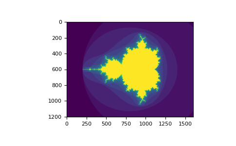
您可以查看以下範例,了解如何使用布林索引來產生曼德博集合的影像。
>>> import numpy as np
>>> import matplotlib.pyplot as plt
>>> def mandelbrot(h, w, maxit=20, r=2):
...     """Returns an image of the Mandelbrot fractal of size (h,w)."""
...     x = np.linspace(-2.5, 1.5, 4*h+1)
...     y = np.linspace(-1.5, 1.5, 3*w+1)
...     A, B = np.meshgrid(x, y)
...     C = A + B*1j
...     z = np.zeros_like(C)
...     divtime = maxit + np.zeros(z.shape, dtype=int)
...
...     for i in range(maxit):
...         z = z**2 + C
...         diverge = abs(z) > r                    # who is diverging
...         div_now = diverge & (divtime == maxit)  # who is diverging now
...         divtime[div_now] = i                    # note when
...         z[diverge] = r                          # avoid diverging too much
...
...     return divtime
>>> plt.clf()
>>> plt.imshow(mandelbrot(400, 400))
第二種使用布林值進行索引的方法更類似於整數索引; 對於陣列的每個維度,我們都給出一個 1D 布林陣列,以選擇我們想要的切片。
>>> a = np.arange(12).reshape(3, 4)
>>> b1 = np.array([False, True, True])         # first dim selection
>>> b2 = np.array([True, False, True, False])  # second dim selection
>>>
>>> a[b1, :]                                   # selecting rows
array([[ 4,  5,  6,  7],
       [ 8,  9, 10, 11]])
>>>
>>> a[b1]                                      # same thing
array([[ 4,  5,  6,  7],
       [ 8,  9, 10, 11]])
>>>
>>> a[:, b2]                                   # selecting columns
array([[ 0,  2],
       [ 4,  6],
       [ 8, 10]])
>>>
>>> a[b1, b2]                                  # a weird thing to do
array([ 4, 10])
請注意,1D 布林陣列的長度必須與您要切片的維度(或軸)的長度一致。 在先前的範例中,b1 的長度為 3(a 中的 *列* 數),而 b2(長度為 4)適用於索引 a 的第二軸(欄)。
ix_() 函式#
ix_ 函式可用於組合不同的向量,以便獲得每個 n 元組的結果。 例如,如果您想計算從向量 a、b 和 c 中取得的所有三元組的 a+b*c。
>>> a = np.array([2, 3, 4, 5])
>>> b = np.array([8, 5, 4])
>>> c = np.array([5, 4, 6, 8, 3])
>>> ax, bx, cx = np.ix_(a, b, c)
>>> ax
array([[[2]],

       [[3]],

       [[4]],

       [[5]]])
>>> bx
array([[[8],
        [5],
        [4]]])
>>> cx
array([[[5, 4, 6, 8, 3]]])
>>> ax.shape, bx.shape, cx.shape
((4, 1, 1), (1, 3, 1), (1, 1, 5))
>>> result = ax + bx * cx
>>> result
array([[[42, 34, 50, 66, 26],
        [27, 22, 32, 42, 17],
        [22, 18, 26, 34, 14]],

       [[43, 35, 51, 67, 27],
        [28, 23, 33, 43, 18],
        [23, 19, 27, 35, 15]],

       [[44, 36, 52, 68, 28],
        [29, 24, 34, 44, 19],
        [24, 20, 28, 36, 16]],

       [[45, 37, 53, 69, 29],
        [30, 25, 35, 45, 20],
        [25, 21, 29, 37, 17]]])
>>> result[3, 2, 4]
17
>>> a[3] + b[2] * c[4]
17
您也可以如下實作 reduce。
>>> def ufunc_reduce(ufct, *vectors):
...    vs = np.ix_(*vectors)
...    r = ufct.identity
...    for v in vs:
...        r = ufct(r, v)
...    return r
然後將其用作
>>> ufunc_reduce(np.add, a, b, c)
array([[[15, 14, 16, 18, 13],
        [12, 11, 13, 15, 10],
        [11, 10, 12, 14,  9]],

       [[16, 15, 17, 19, 14],
        [13, 12, 14, 16, 11],
        [12, 11, 13, 15, 10]],

       [[17, 16, 18, 20, 15],
        [14, 13, 15, 17, 12],
        [13, 12, 14, 16, 11]],

       [[18, 17, 19, 21, 16],
        [15, 14, 16, 18, 13],
        [14, 13, 15, 17, 12]]])
與常規 ufunc.reduce 相比,此版本 reduce 的優點在於,它利用 廣播規則,以避免建立一個參數陣列,其大小為輸出大小乘以向量數量。
使用字串進行索引#
請參閱 結構化陣列。
訣竅與提示#
在此我們提供一份簡短且實用的提示列表。
「自動」重新塑形#
若要變更陣列的維度,您可以省略其中一個大小,然後將自動推導出該大小。
>>> a = np.arange(30)
>>> b = a.reshape((2, -1, 3))  # -1 means "whatever is needed"
>>> b.shape
(2, 5, 3)
>>> b
array([[[ 0,  1,  2],
        [ 3,  4,  5],
        [ 6,  7,  8],
        [ 9, 10, 11],
        [12, 13, 14]],

       [[15, 16, 17],
        [18, 19, 20],
        [21, 22, 23],
        [24, 25, 26],
        [27, 28, 29]]])
向量堆疊#
我們如何從等大小的列向量列表建構 2D 陣列? 在 MATLAB 中,這非常容易:如果 x 和 y 是兩個長度相同的向量,您只需要執行 m=[x;y]。 在 NumPy 中,這透過函式 column_stack、dstack、hstack 和 vstack 實現,具體取決於要進行堆疊的維度。 例如
>>> x = np.arange(0, 10, 2)
>>> y = np.arange(5)
>>> m = np.vstack([x, y])
>>> m
array([[0, 2, 4, 6, 8],
       [0, 1, 2, 3, 4]])
>>> xy = np.hstack([x, y])
>>> xy
array([0, 2, 4, 6, 8, 0, 1, 2, 3, 4])
這些函式在兩個以上維度中的邏輯可能很奇怪。
另請參閱
直方圖#
應用於陣列的 NumPy histogram 函式會傳回一對向量:陣列的直方圖和 bin 邊緣的向量。 請注意:matplotlib 也具有一個用於建構直方圖的函式(稱為 hist,如 Matlab 中所示),該函式與 NumPy 中的函式不同。 主要區別在於 pylab.hist 自動繪製直方圖,而 numpy.histogram 僅產生資料。
>>> import numpy as np
>>> rg = np.random.default_rng(1)
>>> import matplotlib.pyplot as plt
>>> # Build a vector of 10000 normal deviates with variance 0.5^2 and mean 2
>>> mu, sigma = 2, 0.5
>>> v = rg.normal(mu, sigma, 10000)
>>> # Plot a normalized histogram with 50 bins
>>> plt.hist(v, bins=50, density=True)       # matplotlib version (plot)
(array...)
>>> # Compute the histogram with numpy and then plot it
>>> (n, bins) = np.histogram(v, bins=50, density=True)  # NumPy version (no plot)
>>> plt.plot(.5 * (bins[1:] + bins[:-1]), n)
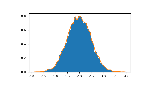
使用 Matplotlib >=3.4,您也可以使用 plt.stairs(n, bins)。