numpy.random.Generator.wald#

方法

random.Generator.wald(mean, scale, size=None)#

從 Wald 或反高斯分佈中抽取樣本。

當 scale 接近無限大時，分佈變得更像高斯分佈。有些參考文獻聲稱 Wald 是平均值等於 1 的反高斯分佈，但這絕非普遍適用。

反高斯分佈最初是在研究布朗運動的關係時被研究的。1956 年，M.C.K. Tweedie 使用了反高斯這個名稱，因為單位距離的行進時間與單位時間內行進的距離之間存在反比關係。

參數:

meanfloat 或 float 的類陣列 (array_like): 分佈平均值，必須 > 0。
scalefloat 或 float 的類陣列 (array_like): 比例參數，必須 > 0。
sizeint 或 int 元組，選用: 輸出形狀。如果給定的形狀是，例如， (m, n, k)，則會抽取 m * n * k 個樣本。如果 size 是 None (預設值)，則如果 mean 和 scale 都是純量，則會傳回單一值。否則，會抽取 np.broadcast(mean, scale).size 個樣本。

傳回值:

註解

Wald 分佈的機率密度函數為

\[P(x;mean,scale) = \sqrt{\frac{scale}{2\pi x^3}}e^ \frac{-scale(x-mean)^2}{2\cdotp mean^2x}\]

如上所述，反高斯分佈首先出現在試圖模擬布朗運動時。它也是 Weibull 分佈在可靠性建模以及股票報酬和利率過程建模中的競爭對手。

參考文獻

[1]

[2]

Chhikara, Raj S. 和 Folks, J. Leroy，“The Inverse Gaussian Distribution: Theory : Methodology, and Applications”，CRC Press，1988。

[3]

範例

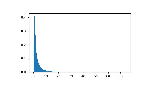
從分佈中抽取值並繪製直方圖

>>> import matplotlib.pyplot as plt
>>> rng = np.random.default_rng()
>>> h = plt.hist(rng.wald(3, 2, 100000), bins=200, density=True)
>>> plt.show()