numpy.random.Generator.power

方法

random.Generator.power(a, size=None)

從具有正指數 a - 1 的冪分佈中抽取 [0, 1] 範圍內的樣本。

也稱為冪函數分佈。

參數:

afloat 或 float 陣列型物件

分佈的參數。必須是非負數。

sizeint 或 int 元組，選用

輸出形狀。如果給定的形狀為，例如 (m, n, k)，則會抽取 m * n * k 個樣本。如果 size 為 None (預設值)，則如果 a 是純量，則會回傳單一值。否則，會抽取 np.array(a).size 個樣本。

回傳值:

outndarray 或 純量

從參數化的冪分佈中抽取的樣本。

拋出:

ValueError

如果 a <= 0。

註解

機率密度函數為

\[P(x; a) = ax^{a-1}, 0 \le x \le 1, a>0.\]

冪函數分佈只是帕雷托分佈的反函數。它也可以被視為 Beta 分佈的特例。

例如，它用於對保險索賠的過度申報進行建模。

參考文獻

[1]

Christian Kleiber, Samuel Kotz, “Statistical size distributions in economics and actuarial sciences”, Wiley, 2003.

[2]

Heckert, N. A. and Filliben, James J. “NIST Handbook 148: Dataplot Reference Manual, Volume 2: Let Subcommands and Library Functions”, National Institute of Standards and Technology Handbook Series, June 2003. https://www.itl.nist.gov/div898/software/dataplot/refman2/auxillar/powpdf.pdf

範例

從分佈中抽取樣本

>>> rng = np.random.default_rng()
>>> a = 5. # shape
>>> samples = 1000
>>> s = rng.power(a, samples)

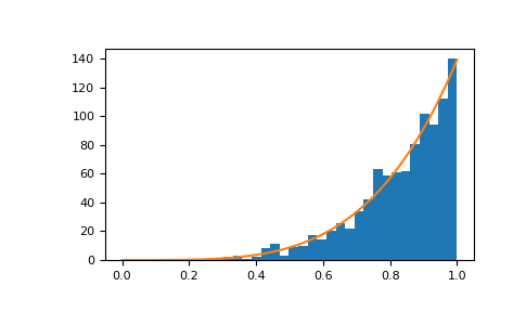
顯示樣本的直方圖，以及機率密度函數

>>> import matplotlib.pyplot as plt
>>> count, bins, _ = plt.hist(s, bins=30)
>>> x = np.linspace(0, 1, 100)
>>> y = a*x**(a-1.)
>>> normed_y = samples*np.diff(bins)[0]*y
>>> plt.plot(x, normed_y)
>>> plt.show()

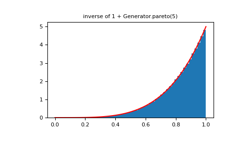
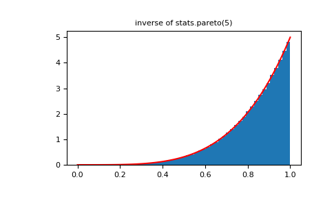
比較冪函數分佈與帕雷托分佈的反函數。

>>> from scipy import stats  
>>> rvs = rng.power(5, 1000000)
>>> rvsp = rng.pareto(5, 1000000)
>>> xx = np.linspace(0,1,100)
>>> powpdf = stats.powerlaw.pdf(xx,5)  

>>> plt.figure()
>>> plt.hist(rvs, bins=50, density=True)
>>> plt.plot(xx,powpdf,'r-')  
>>> plt.title('power(5)')

>>> plt.figure()
>>> plt.hist(1./(1.+rvsp), bins=50, density=True)
>>> plt.plot(xx,powpdf,'r-')  
>>> plt.title('inverse of 1 + Generator.pareto(5)')

>>> plt.figure()
>>> plt.hist(1./(1.+rvsp), bins=50, density=True)
>>> plt.plot(xx,powpdf,'r-')  
>>> plt.title('inverse of stats.pareto(5)')