numpy.random.Generator.lognormal

方法

random.Generator.lognormal(mean=0.0, sigma=1.0, size=None)

從對數常態分佈中抽取樣本。

從具有指定均值、標準差和陣列形狀的對數常態分佈中抽取樣本。請注意，均值和標準差不是分佈本身的值，而是其所源自的底層常態分佈的值。

參數:

meanfloat 或 float 類陣列，選用

底層常態分佈的均值。預設值為 0。

sigmafloat 或 float 類陣列，選用

底層常態分佈的標準差。必須為非負數。預設值為 1。

sizeint 或 int 元組，選用

輸出形狀。如果給定的形狀為，例如，(m, n, k)，則會抽取 m * n * k 個樣本。如果 size 為 None (預設值)，則當 mean 和 sigma 均為純量時，會傳回單一值。否則，會抽取 np.broadcast(mean, sigma).size 個樣本。

傳回值:

outndarray 或 純量

從參數化的對數常態分佈中抽取的樣本。

另請參閱

scipy.stats.lognorm

機率密度函數、分佈、累積密度函數等。

註解

若變數 x 具有對數常態分佈，則 log(x) 為常態分佈。對數常態分佈的機率密度函數為

\[p(x) = \frac{1}{\sigma x \sqrt{2\pi}} e^{(-\frac{(ln(x)-\mu)^2}{2\sigma^2})}\]

其中 \(\mu\) 是變數的常態分佈對數的均值，而 \(\sigma\) 是標準差。如果隨機變數是大量獨立、同分佈變數的乘積，則會產生對數常態分佈，這與變數是大量獨立、同分佈變數的總和時產生常態分佈的方式相同。

參考文獻

[1]

Limpert, E., Stahel, W. A., and Abbt, M., “Log-normal Distributions across the Sciences: Keys and Clues,” BioScience, Vol. 51, No. 5, May, 2001. https://stat.ethz.ch/~stahel/lognormal/bioscience.pdf

[2]

Reiss, R.D. and Thomas, M., “Statistical Analysis of Extreme Values,” Basel: Birkhauser Verlag, 2001, pp. 31-32.

範例

從分佈中抽取樣本

>>> rng = np.random.default_rng()
>>> mu, sigma = 3., 1. # mean and standard deviation
>>> s = rng.lognormal(mu, sigma, 1000)

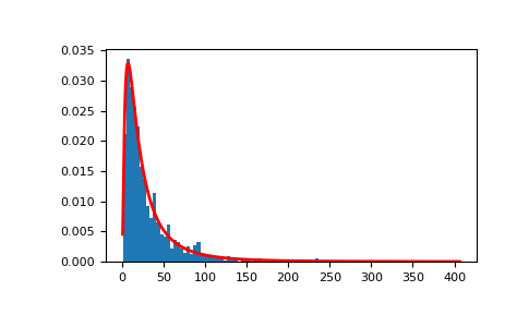
顯示樣本的直方圖，以及機率密度函數

>>> import matplotlib.pyplot as plt
>>> count, bins, _ = plt.hist(s, 100, density=True, align='mid')

>>> x = np.linspace(min(bins), max(bins), 10000)
>>> pdf = (np.exp(-(np.log(x) - mu)**2 / (2 * sigma**2))
...        / (x * sigma * np.sqrt(2 * np.pi)))

>>> plt.plot(x, pdf, linewidth=2, color='r')
>>> plt.axis('tight')
>>> plt.show()

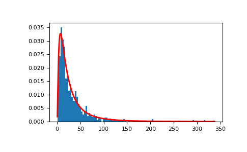
示範從均勻分佈中抽取隨機樣本的乘積，可以很好地由對數常態機率密度函數擬合。

>>> # Generate a thousand samples: each is the product of 100 random
>>> # values, drawn from a normal distribution.
>>> rng = rng
>>> b = []
>>> for i in range(1000):
...    a = 10. + rng.standard_normal(100)
...    b.append(np.prod(a))

>>> b = np.array(b) / np.min(b) # scale values to be positive
>>> count, bins, _ = plt.hist(b, 100, density=True, align='mid')
>>> sigma = np.std(np.log(b))
>>> mu = np.mean(np.log(b))

>>> x = np.linspace(min(bins), max(bins), 10000)
>>> pdf = (np.exp(-(np.log(x) - mu)**2 / (2 * sigma**2))
...        / (x * sigma * np.sqrt(2 * np.pi)))

>>> plt.plot(x, pdf, color='r', linewidth=2)
>>> plt.show()