
MNIST 上的深度學習#
本教學示範如何建構一個簡單的前饋神經網路(具有一個隱藏層),並從頭開始使用 NumPy 訓練它,以識別手寫數字影像。
您的深度學習模型 — 最基本的人工神經網路之一,類似於原始的多層感知器 — 將學習從MNIST資料集中分類 0 到 9 的數字。該資料集包含 60,000 個訓練影像和 10,000 個測試影像以及對應的標籤。每個訓練和測試影像的大小為 784(或 28x28 像素)— 這將是您神經網路的輸入。
根據影像輸入及其標籤(監督式學習),您的神經網路將接受訓練,以使用前向傳播和反向傳播(反向模式微分)來學習它們的特徵。網路的最終輸出是一個包含 10 個分數的向量 — 每個手寫數字影像一個。您還將評估您的模型在測試集上分類影像的效果。
本教學改編自 Andrew Trask 的作品(經作者許可)。
先決條件#
讀者應具備 Python、NumPy 陣列操作和線性代數的一些知識。此外,您應該熟悉深度學習的主要概念。
為了刷新記憶,您可以參加 Python 和 n 維陣列上的線性代數教學。
建議您閱讀 Yann LeCun、Yoshua Bengio 和 Geoffrey Hinton 於 2015 年發表的深度學習論文,他們被認為是該領域的先驅。您也應該考慮閱讀 Andrew Trask 的 Grokking Deep Learning,該書使用 NumPy 教學深度學習。
除了 NumPy 之外,您還將使用以下 Python 標準模組進行資料載入和處理
urllib用於 URL 處理request用於 URL 開啟gzip用於 gzip 檔案解壓縮pickle用於處理 pickle 檔案格式以及
Matplotlib 用於資料視覺化
本教學可以在隔離環境中在本機執行,例如 Virtualenv 或 conda。您可以使用 Jupyter Notebook 或 JupyterLab 來執行每個筆記本儲存格。別忘了設定 NumPy 和 Matplotlib。
目錄#
載入 MNIST 資料集
預處理資料集
從頭開始建構和訓練小型神經網路
後續步驟
1. 載入 MNIST 資料集#
在本節中,您將下載最初儲存在 Yann LeCun 的網站中的壓縮 MNIST 資料集檔案。然後,您將使用內建的 Python 模組將它們轉換為 4 個 NumPy 陣列類型檔案。最後,您將陣列分成訓練集和測試集。
1. 定義一個變數,以列表形式儲存 MNIST 資料集的訓練/測試影像/標籤名稱
data_sources = {
    "training_images": "train-images-idx3-ubyte.gz",  # 60,000 training images.
    "test_images": "t10k-images-idx3-ubyte.gz",  # 10,000 test images.
    "training_labels": "train-labels-idx1-ubyte.gz",  # 60,000 training labels.
    "test_labels": "t10k-labels-idx1-ubyte.gz",  # 10,000 test labels.
}
2. 載入資料。首先檢查資料是否在本機儲存;如果沒有,則下載資料。
import requests
import os

data_dir = "../_data"
os.makedirs(data_dir, exist_ok=True)

base_url = "https://github.com/rossbar/numpy-tutorial-data-mirror/blob/main/"

for fname in data_sources.values():
    fpath = os.path.join(data_dir, fname)
    if not os.path.exists(fpath):
        print("Downloading file: " + fname)
        resp = requests.get(base_url + fname, stream=True, **request_opts)
        resp.raise_for_status()  # Ensure download was succesful
        with open(fpath, "wb") as fh:
            for chunk in resp.iter_content(chunk_size=128):
                fh.write(chunk)
3. 解壓縮 4 個檔案並建立 4 個 ndarray,將它們儲存到字典中。每個原始影像的大小為 28x28,而神經網路通常期望 1D 向量輸入;因此,您也需要將影像重塑為 28 乘以 28 (784)。
import gzip
import numpy as np

mnist_dataset = {}

# Images
for key in ("training_images", "test_images"):
    with gzip.open(os.path.join(data_dir, data_sources[key]), "rb") as mnist_file:
        mnist_dataset[key] = np.frombuffer(
            mnist_file.read(), np.uint8, offset=16
        ).reshape(-1, 28 * 28)
# Labels
for key in ("training_labels", "test_labels"):
    with gzip.open(os.path.join(data_dir, data_sources[key]), "rb") as mnist_file:
        mnist_dataset[key] = np.frombuffer(mnist_file.read(), np.uint8, offset=8)
4. 使用 x 表示資料和 y 表示標籤的標準符號,將資料分成訓練集和測試集,將訓練集和測試集影像稱為 x_train 和 x_test,標籤稱為 y_train 和 y_test
x_train, y_train, x_test, y_test = (
    mnist_dataset["training_images"],
    mnist_dataset["training_labels"],
    mnist_dataset["test_images"],
    mnist_dataset["test_labels"],
)
5. 您可以確認影像陣列的形狀對於訓練集和測試集分別為 (60000, 784) 和 (10000, 784),而標籤為 (60000,) 和 (10000,)
print(
    "The shape of training images: {} and training labels: {}".format(
        x_train.shape, y_train.shape
    )
)
print(
    "The shape of test images: {} and test labels: {}".format(
        x_test.shape, y_test.shape
    )
)
The shape of training images: (60000, 784) and training labels: (60000,)
The shape of test images: (10000, 784) and test labels: (10000,)
6. 您可以使用 Matplotlib 檢查一些影像
import matplotlib.pyplot as plt
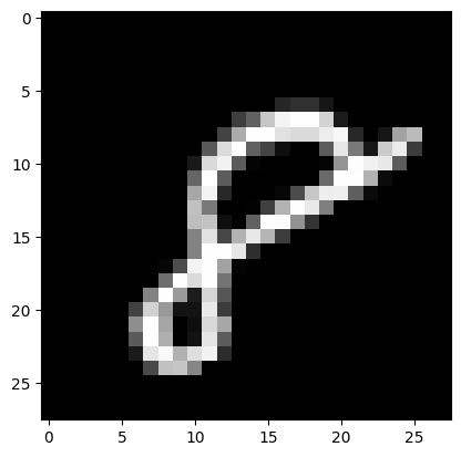
# Take the 60,000th image (indexed at 59,999) from the training set,
# reshape from (784, ) to (28, 28) to have a valid shape for displaying purposes.
mnist_image = x_train[59999, :].reshape(28, 28)
# Set the color mapping to grayscale to have a black background.
plt.imshow(mnist_image, cmap="gray")
# Display the image.
plt.show()
# Display 5 random images from the training set.
num_examples = 5
seed = 147197952744
rng = np.random.default_rng(seed)

fig, axes = plt.subplots(1, num_examples)
for sample, ax in zip(rng.choice(x_train, size=num_examples, replace=False), axes):
    ax.imshow(sample.reshape(28, 28), cmap="gray")
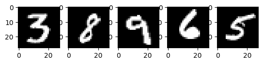
以上是從 MNIST 訓練集中擷取的五個影像。顯示了各種手繪阿拉伯數字,確切值在每次程式碼執行時隨機選擇。
注意: 您也可以透過列印
x_train[59999]將範例影像視覺化為陣列。這裡,59999是您的第 60,000 個訓練影像範例(0將是您的第一個)。您的輸出將非常長,並且應包含 8 位元整數的陣列... 0, 0, 38, 48, 48, 22, 0, 0, 0, 0, 0, 0, 0, 0, 0, 0, 0, 0, 0, 0, 0, 0, 0, 0, 0, 0, 0, 62, 97, 198, 243, 254, 254, 212, 27, 0, 0, 0, 0, ...
# Display the label of the 60,000th image (indexed at 59,999) from the training set.
y_train[59999]
np.uint8(8)
2. 預處理資料#
神經網路可以使用張量(多維陣列)形式的浮點類型輸入。在預處理資料時,您應考慮以下流程:向量化和轉換為浮點格式。
由於 MNIST 資料已向量化,並且陣列的 dtype 為 uint8,因此您的下一個挑戰是將它們轉換為浮點格式,例如 float64(雙精度)
實際上,您可以根據您的目標使用不同類型的浮點精度,並且您可以在 Nvidia 和 Google Cloud 部落格文章中找到有關此的更多資訊。
將影像資料轉換為浮點格式#
影像資料包含編碼在 [0, 255] 區間中的 8 位元整數,顏色值介於 0 和 255 之間。
您將透過將它們除以 255,將它們正規化為 [0, 1] 區間中的浮點陣列。
1. 檢查向量化影像資料是否為 uint8 類型
print("The data type of training images: {}".format(x_train.dtype))
print("The data type of test images: {}".format(x_test.dtype))
The data type of training images: uint8
The data type of test images: uint8
2. 透過將陣列除以 255 來正規化陣列(因此將資料類型從 uint8 提升為 float64),然後將訓練和測試影像資料變數 — x_train 和 x_test — 分別指派給 training_images 和 train_labels。為了減少本範例中的模型訓練和評估時間,將僅使用訓練和測試影像的子集。 training_images 和 test_images 都將僅包含 1,000 個範例,分別來自完整資料集 60,000 個和 10,000 個影像。這些值可以透過變更下方的 training_sample 和 test_sample 來控制,最多可達其最大值 60,000 和 10,000。
training_sample, test_sample = 1000, 1000
training_images = x_train[0:training_sample] / 255
test_images = x_test[0:test_sample] / 255
3. 確認影像資料已變更為浮點格式
print("The data type of training images: {}".format(training_images.dtype))
print("The data type of test images: {}".format(test_images.dtype))
The data type of training images: float64
The data type of test images: float64
注意: 您也可以透過在筆記本儲存格中列印
training_images[0]來檢查正規化是否成功。您的長輸出應包含浮點數的陣列... 0. , 0. , 0.01176471, 0.07058824, 0.07058824, 0.07058824, 0.49411765, 0.53333333, 0.68627451, 0.10196078, 0.65098039, 1. , 0.96862745, 0.49803922, 0. , ...
透過類別/獨熱編碼將標籤轉換為浮點數#
您將使用獨熱編碼將每個數字標籤嵌入為全零向量,其中包含 np.zeros(),並為標籤索引放置 1。因此,您的標籤資料將是陣列,其中每個影像標籤的位置都有 1.0(或 1.)。
由於總共有 10 個標籤(從 0 到 9),因此您的陣列將如下所示
array([0., 0., 0., 0., 0., 1., 0., 0., 0., 0.])
1. 確認影像標籤資料是 dtype 為 uint8 的整數
print("The data type of training labels: {}".format(y_train.dtype))
print("The data type of test labels: {}".format(y_test.dtype))
The data type of training labels: uint8
The data type of test labels: uint8
2. 定義一個對陣列執行獨熱編碼的函式
def one_hot_encoding(labels, dimension=10):
    # Define a one-hot variable for an all-zero vector
    # with 10 dimensions (number labels from 0 to 9).
    one_hot_labels = labels[..., None] == np.arange(dimension)[None]
    # Return one-hot encoded labels.
    return one_hot_labels.astype(np.float64)
3. 編碼標籤並將值指派給新變數
training_labels = one_hot_encoding(y_train[:training_sample])
test_labels = one_hot_encoding(y_test[:test_sample])
4. 檢查資料類型是否已變更為浮點數
print("The data type of training labels: {}".format(training_labels.dtype))
print("The data type of test labels: {}".format(test_labels.dtype))
The data type of training labels: float64
The data type of test labels: float64
5. 檢查一些編碼標籤
print(training_labels[0])
print(training_labels[1])
print(training_labels[2])
[0. 0. 0. 0. 0. 1. 0. 0. 0. 0.]
[1. 0. 0. 0. 0. 0. 0. 0. 0. 0.]
[0. 0. 0. 0. 1. 0. 0. 0. 0. 0.]
…並與原始標籤進行比較
print(y_train[0])
print(y_train[1])
print(y_train[2])
5
0
4
您已完成資料集的準備。
3. 從頭開始建構和訓練小型神經網路#
在本節中,您將熟悉深度學習模型基本建構區塊的一些高階概念。您可以參考原始的深度學習研究出版物以取得更多資訊。
之後,您將在 Python 和 NumPy 中建構簡單深度學習模型的建構區塊,並訓練它學習以一定的準確度從 MNIST 資料集中識別手寫數字。
使用 NumPy 的神經網路建構區塊#
層:這些建構區塊充當資料篩選器 — 它們處理資料並從輸入中學習表示法,以更好地預測目標輸出。
您將在模型中使用 1 個隱藏層來向前傳遞輸入(前向傳播)並向後傳播損失函數的梯度/誤差導數(反向傳播)。這些是輸入層、隱藏層和輸出層。
在隱藏(中間)層和輸出(最後)層中,神經網路模型將計算輸入的加權總和。為了計算此過程,您將使用 NumPy 的矩陣乘法函數(「點乘」或
np.dot(layer, weights))。注意: 為了簡化,本範例中省略了偏差項(沒有
np.dot(layer, weights) + bias)。權重:這些是重要的可調整參數,神經網路透過向前和向後傳播資料來微調。它們透過稱為梯度下降的過程進行最佳化。在模型訓練開始之前,權重會使用 NumPy 的
Generator.random()隨機初始化。最佳權重應在訓練集和測試集上產生最高的預測準確度和最低的誤差。
啟動函數:深度學習模型能夠確定輸入和輸出之間的非線性關係,並且這些非線性函數通常應用於每層的輸出。
您將使用整流線性單元 (ReLU) 作為隱藏層的輸出(例如,
relu(np.dot(layer, weights)))。-
在本範例中,您將使用一種稱為 dropout 的方法 — 稀釋 — 它隨機將層中的許多特徵設定為 0。您將使用 NumPy 的
Generator.integers()方法定義它,並將其應用於網路的隱藏層。 損失函數:計算透過比較影像標籤(真值)與最終層輸出中的預測值來確定預測的品質。
為了簡化,您將使用基本的總平方誤差,使用 NumPy 的
np.sum()函數(例如,np.sum((final_layer_output - image_labels) ** 2))。準確度:此指標衡量網路預測其未見資料的能力的準確度。
模型架構和訓練摘要#
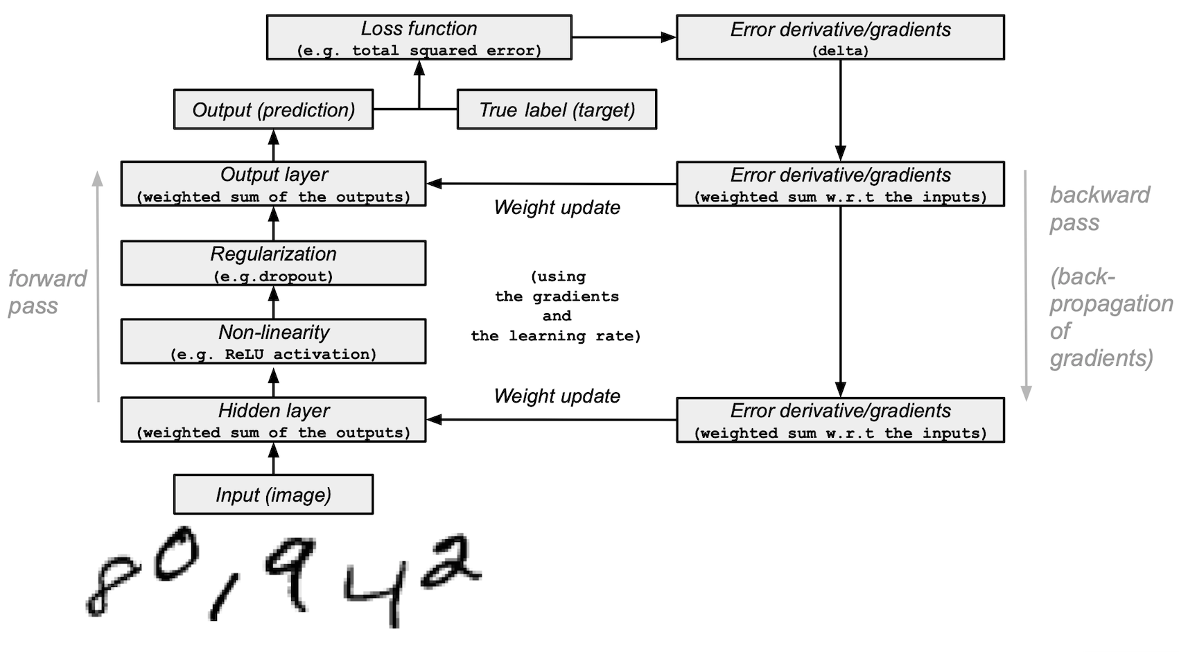
以下是神經網路模型架構和訓練過程的摘要
輸入層:
它是網路的輸入 — 先前預處理的資料,從
training_images載入到layer_0中。隱藏(中間)層:
layer_1取得前一層的輸出,並使用 NumPy 的np.dot()將輸入與權重 (weights_1) 執行矩陣乘法。然後,此輸出透過 ReLU 啟動函數進行非線性化,然後應用 dropout 以協助解決過度擬合問題。
輸出(最後)層:
layer_2擷取layer_1的輸出,並使用weights_2重複相同的「點乘」過程。最終輸出傳回每個 0-9 數字標籤的 10 個分數。網路模型以大小為 10 的層結束 — 10 維向量。
前向傳播、反向傳播、訓練迴圈:
在模型訓練開始時,您的網路隨機初始化權重,並透過隱藏層和輸出層向前饋送輸入資料。此過程是前向傳遞或前向傳播。
然後,網路將損失函數的「訊號」向後傳播通過隱藏層,並在學習率參數的幫助下調整權重值(稍後將詳細介紹)。
組成模型並開始訓練和測試#
在涵蓋了主要的深度學習概念和神經網路架構之後,讓我們編寫程式碼。
1. 我們將從建立新的隨機數產生器開始,為再現性提供種子
seed = 884736743
rng = np.random.default_rng(seed)
2. 對於隱藏層,定義用於前向傳播的 ReLU 啟動函數和將在反向傳播期間使用的 ReLU 導數
# Define ReLU that returns the input if it's positive and 0 otherwise.
def relu(x):
    return (x >= 0) * x


# Set up a derivative of the ReLU function that returns 1 for a positive input
# and 0 otherwise.
def relu2deriv(output):
    return output >= 0
3. 設定某些超參數的預設值,例如
學習率:
learning_rate— 有助於限制權重更新的幅度,以防止它們過度校正。Epoch(迭代):
epochs— 資料通過網路的完整傳遞次數(前向和反向傳播)。此參數可能會對結果產生正面或負面影響。迭代次數越高,學習過程可能需要的時間越長。由於這是一項計算密集型任務,因此我們選擇了非常少的 epoch 數 (20)。為了獲得有意義的結果,您應該選擇更大的數字。網路中隱藏(中間)層的大小:
hidden_size— 隱藏層的不同大小可能會影響訓練和測試期間的結果。輸入大小:
pixels_per_image— 您已確定影像輸入為 784 (28x28)(以像素為單位)。標籤數量:
num_labels— 指示輸出層的輸出數量,其中發生 10 個(0 到 9)手寫數字標籤的預測。
learning_rate = 0.005
epochs = 20
hidden_size = 100
pixels_per_image = 784
num_labels = 10
4. 使用隨機值初始化將在隱藏層和輸出層中使用的權重向量
weights_1 = 0.2 * rng.random((pixels_per_image, hidden_size)) - 0.1
weights_2 = 0.2 * rng.random((hidden_size, num_labels)) - 0.1
5. 使用訓練迴圈設定神經網路的學習實驗,並開始訓練過程。請注意,在每個 epoch 都會針對測試集評估模型,以追蹤其在訓練 epoch 中的效能。
開始訓練過程
# To store training and test set losses and accurate predictions
# for visualization.
store_training_loss = []
store_training_accurate_pred = []
store_test_loss = []
store_test_accurate_pred = []

# This is a training loop.
# Run the learning experiment for a defined number of epochs (iterations).
for j in range(epochs):

    #################
    # Training step #
    #################

    # Set the initial loss/error and the number of accurate predictions to zero.
    training_loss = 0.0
    training_accurate_predictions = 0

    # For all images in the training set, perform a forward pass
    # and backpropagation and adjust the weights accordingly.
    for i in range(len(training_images)):
        # Forward propagation/forward pass:
        # 1. The input layer:
        #    Initialize the training image data as inputs.
        layer_0 = training_images[i]
        # 2. The hidden layer:
        #    Take in the training image data into the middle layer by
        #    matrix-multiplying it by randomly initialized weights.
        layer_1 = np.dot(layer_0, weights_1)
        # 3. Pass the hidden layer's output through the ReLU activation function.
        layer_1 = relu(layer_1)
        # 4. Define the dropout function for regularization.
        dropout_mask = rng.integers(low=0, high=2, size=layer_1.shape)
        # 5. Apply dropout to the hidden layer's output.
        layer_1 *= dropout_mask * 2
        # 6. The output layer:
        #    Ingest the output of the middle layer into the the final layer
        #    by matrix-multiplying it by randomly initialized weights.
        #    Produce a 10-dimension vector with 10 scores.
        layer_2 = np.dot(layer_1, weights_2)

        # Backpropagation/backward pass:
        # 1. Measure the training error (loss function) between the actual
        #    image labels (the truth) and the prediction by the model.
        training_loss += np.sum((training_labels[i] - layer_2) ** 2)
        # 2. Increment the accurate prediction count.
        training_accurate_predictions += int(
            np.argmax(layer_2) == np.argmax(training_labels[i])
        )
        # 3. Differentiate the loss function/error.
        layer_2_delta = training_labels[i] - layer_2
        # 4. Propagate the gradients of the loss function back through the hidden layer.
        layer_1_delta = np.dot(weights_2, layer_2_delta) * relu2deriv(layer_1)
        # 5. Apply the dropout to the gradients.
        layer_1_delta *= dropout_mask
        # 6. Update the weights for the middle and input layers
        #    by multiplying them by the learning rate and the gradients.
        weights_1 += learning_rate * np.outer(layer_0, layer_1_delta)
        weights_2 += learning_rate * np.outer(layer_1, layer_2_delta)

    # Store training set losses and accurate predictions.
    store_training_loss.append(training_loss)
    store_training_accurate_pred.append(training_accurate_predictions)

    ###################
    # Evaluation step #
    ###################

    # Evaluate model performance on the test set at each epoch.

    # Unlike the training step, the weights are not modified for each image
    # (or batch). Therefore the model can be applied to the test images in a
    # vectorized manner, eliminating the need to loop over each image
    # individually:

    results = relu(test_images @ weights_1) @ weights_2

    # Measure the error between the actual label (truth) and prediction values.
    test_loss = np.sum((test_labels - results) ** 2)

    # Measure prediction accuracy on test set
    test_accurate_predictions = np.sum(
        np.argmax(results, axis=1) == np.argmax(test_labels, axis=1)
    )

    # Store test set losses and accurate predictions.
    store_test_loss.append(test_loss)
    store_test_accurate_pred.append(test_accurate_predictions)

    # Summarize error and accuracy metrics at each epoch
    print(
        (
            f"Epoch: {j}\n"
            f"  Training set error: {training_loss / len(training_images):.3f}\n"
            f"  Training set accuracy: {training_accurate_predictions / len(training_images)}\n"
            f"  Test set error: {test_loss / len(test_images):.3f}\n"
            f"  Test set accuracy: {test_accurate_predictions / len(test_images)}"
        )
    )
Epoch: 0
  Training set error: 0.898
  Training set accuracy: 0.397
  Test set error: 0.680
  Test set accuracy: 0.582
Epoch: 1
  Training set error: 0.656
  Training set accuracy: 0.633
  Test set error: 0.607
  Test set accuracy: 0.641
Epoch: 2
  Training set error: 0.592
  Training set accuracy: 0.68
  Test set error: 0.569
  Test set accuracy: 0.679
Epoch: 3
  Training set error: 0.556
  Training set accuracy: 0.7
  Test set error: 0.541
  Test set accuracy: 0.708
Epoch: 4
  Training set error: 0.534
  Training set accuracy: 0.732
  Test set error: 0.526
  Test set accuracy: 0.729
Epoch: 5
  Training set error: 0.515
  Training set accuracy: 0.715
  Test set error: 0.500
  Test set accuracy: 0.739
Epoch: 6
  Training set error: 0.495
  Training set accuracy: 0.748
  Test set error: 0.487
  Test set accuracy: 0.753
Epoch: 7
  Training set error: 0.483
  Training set accuracy: 0.769
  Test set error: 0.486
  Test set accuracy: 0.747
Epoch: 8
  Training set error: 0.473
  Training set accuracy: 0.776
  Test set error: 0.473
  Test set accuracy: 0.752
Epoch: 9
  Training set error: 0.460
  Training set accuracy: 0.788
  Test set error: 0.462
  Test set accuracy: 0.762
Epoch: 10
  Training set error: 0.465
  Training set accuracy: 0.769
  Test set error: 0.462
  Test set accuracy: 0.767
Epoch: 11
  Training set error: 0.443
  Training set accuracy: 0.801
  Test set error: 0.456
  Test set accuracy: 0.775
Epoch: 12
  Training set error: 0.448
  Training set accuracy: 0.795
  Test set error: 0.455
  Test set accuracy: 0.772
Epoch: 13
  Training set error: 0.438
  Training set accuracy: 0.787
  Test set error: 0.453
  Test set accuracy: 0.778
Epoch: 14
  Training set error: 0.446
  Training set accuracy: 0.791
  Test set error: 0.450
  Test set accuracy: 0.779
Epoch: 15
  Training set error: 0.441
  Training set accuracy: 0.788
  Test set error: 0.452
  Test set accuracy: 0.772
Epoch: 16
  Training set error: 0.437
  Training set accuracy: 0.786
  Test set error: 0.453
  Test set accuracy: 0.772
Epoch: 17
  Training set error: 0.436
  Training set accuracy: 0.794
  Test set error: 0.449
  Test set accuracy: 0.778
Epoch: 18
  Training set error: 0.433
  Training set accuracy: 0.801
  Test set error: 0.450
  Test set accuracy: 0.774
Epoch: 19
  Training set error: 0.429
  Training set accuracy: 0.785
  Test set error: 0.436
  Test set accuracy: 0.784
訓練過程可能需要幾分鐘,具體取決於許多因素,例如您執行實驗的機器的處理能力和 epoch 數量。為了減少等待時間,您可以將 epoch(迭代)變數從 100 變更為較低的數字,重設執行時間(這將重設權重),然後再次執行筆記本儲存格。
在執行上面的儲存格後,您可以視覺化此訓練過程實例的訓練集和測試集誤差和準確度。
epoch_range = np.arange(epochs) + 1  # Starting from 1

# The training set metrics.
training_metrics = {
    "accuracy": np.asarray(store_training_accurate_pred) / len(training_images),
    "error": np.asarray(store_training_loss) / len(training_images),
}

# The test set metrics.
test_metrics = {
    "accuracy": np.asarray(store_test_accurate_pred) / len(test_images),
    "error": np.asarray(store_test_loss) / len(test_images),
}

# Display the plots.
fig, axes = plt.subplots(nrows=1, ncols=2, figsize=(15, 5))
for ax, metrics, title in zip(
    axes, (training_metrics, test_metrics), ("Training set", "Test set")
):
    # Plot the metrics
    for metric, values in metrics.items():
        ax.plot(epoch_range, values, label=metric.capitalize())
    ax.set_title(title)
    ax.set_xlabel("Epochs")
    ax.legend()
plt.show()
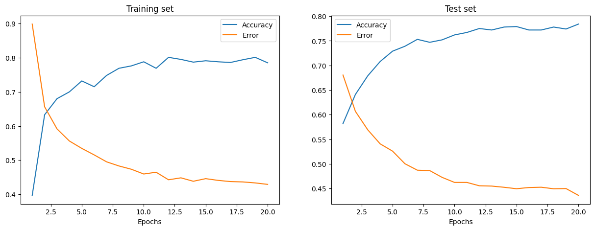
訓練和測試誤差如上圖所示,分別位於左圖和右圖中。隨著 Epoch 數量的增加,總誤差會減少,準確度會提高。
您的模型在訓練和測試期間達到的準確度可能有些合理,但您也可能會發現誤差率相當高。
為了減少訓練和測試期間的誤差,您可以考慮將簡單的損失函數變更為例如類別交叉熵。下面討論了其他可能的解決方案。
後續步驟#
您已學習如何從頭開始僅使用 NumPy 建構和訓練簡單的前饋神經網路,以分類手寫 MNIST 數字。
為了進一步增強和最佳化您的神經網路模型,您可以考慮以下混合方法之一
將訓練樣本大小從 1,000 增加到更高的數字(最多 60,000)。
使用小批量並降低學習率。
透過引入更多隱藏層來改變架構,使網路更深。
引入卷積層:將前饋網路替換為卷積神經網路架構。
引入驗證集,以對模型擬合進行公正的評估。
應用批次正規化,以實現更快、更穩定的訓練。
調整其他參數,例如學習率和隱藏層大小。
從頭開始使用 NumPy 建構神經網路是了解更多關於 NumPy 和深度學習的好方法。但是,對於實際應用,您應該使用專門的框架 — 例如 PyTorch、JAX、TensorFlow 或 MXNet — 這些框架提供類似 NumPy 的 API,具有內建的自動微分和 GPU 支援,並且專為高效能數值計算和機器學習而設計。
最後,在開發機器學習模型時,您應該考慮潛在的倫理問題,並應用實務來避免或減輕這些問題
使用模型卡記錄經過訓練的模型 - 請參閱 Margaret Mitchell 等人的模型報告模型卡論文。
使用資料表記錄資料集 - 請參閱 Timnit Gebru 等人的資料集資料表論文)。
如需更多資源,請參閱 Rachel Thomas 的這篇部落格文章和 Radical AI podcast。
(感謝 hsjeong5 示範如何在不使用外部函式庫的情況下下載 MNIST。)