
X 光影像處理#
本教學示範如何使用 NumPy、imageio、Matplotlib 和 SciPy 讀取和處理 X 光影像。您將學習如何載入醫療影像、聚焦於特定部分,並使用 高斯、拉普拉斯-高斯、索貝爾 和 坎尼 濾波器進行邊緣偵測,以視覺化方式比較它們。
X 光影像分析可以成為您的資料分析和 機器學習工作流程 的一部分,例如,當您正在建立一個演算法,以協助 偵測肺炎,作為 Kaggle 競賽 的一部分。在醫療保健產業中,醫療影像處理和分析尤其重要,因為估計影像佔了 至少 90% 的所有醫療數據。
您將使用來自 ChestX-ray8 資料集的放射影像,該資料集由 美國國家衛生研究院 (NIH) 提供。 ChestX-ray8 包含超過 100,000 張來自 30,000 多名患者的 PNG 格式去識別化 X 光影像。您可以在 NIH 的公共 Box 儲存庫 的 /images 資料夾中找到 ChestX-ray8 的檔案。(如需更多詳細資訊,請參閱 2017 年在 CVPR(電腦視覺會議)上發表的 研究論文。)
為了您的方便,少量 PNG 影像已儲存到本教學的儲存庫中的 tutorial-x-ray-image-processing/ 下,因為 ChestX-ray8 包含數 GB 的資料,您可能會發現批量下載它具有挑戰性。

準備條件#
讀者應具備 Python、NumPy 陣列和 Matplotlib 的一些知識。為了喚醒記憶,您可以學習 Python 和 Matplotlib PyPlot 教學,以及 NumPy 快速入門。
本教學使用以下套件
imageio 用於讀取和寫入影像資料。醫療保健產業通常使用 DICOM 格式進行醫療影像處理,而 imageio 應該非常適合讀取該格式。為了簡化,在本教學中,您將使用 PNG 檔案。
Matplotlib 用於資料視覺化。
本教學可以在隔離環境中本地執行,例如 Virtualenv 或 conda。您可以使用 Jupyter Notebook 或 JupyterLab 來執行每個筆記本單元格。
目錄#
使用
imageio檢查 X 光片將影像組合成多維陣列以展示進展
使用 Laplacian-Gaussian、高斯梯度、Sobel 和 Canny 濾波器進行邊緣偵測
使用
np.where()將遮罩應用於 X 光片比較結果
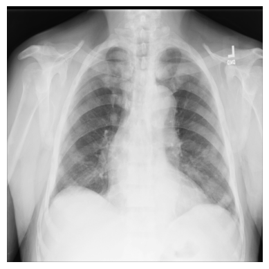
使用 imageio 檢查 X 光片#
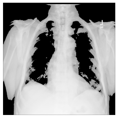
讓我們從一個簡單的範例開始,僅使用 ChestX-ray8 資料集中的一張 X 光影像。
檔案 — 00000011_001.png — 已為您下載並儲存在 /tutorial-x-ray-image-processing 資料夾中。
1. 使用 imageio 載入影像
import os
import imageio

DIR = "tutorial-x-ray-image-processing"

xray_image = imageio.v3.imread(os.path.join(DIR, "00000011_001.png"))
2. 檢查其形狀是否為 1024x1024 像素,以及陣列是否由 8 位元整數組成
print(xray_image.shape)
print(xray_image.dtype)
(1024, 1024)
uint8
3. 匯入 matplotlib 並以灰階色譜顯示影像
import matplotlib.pyplot as plt

plt.imshow(xray_image, cmap="gray")
plt.axis("off")
plt.show()
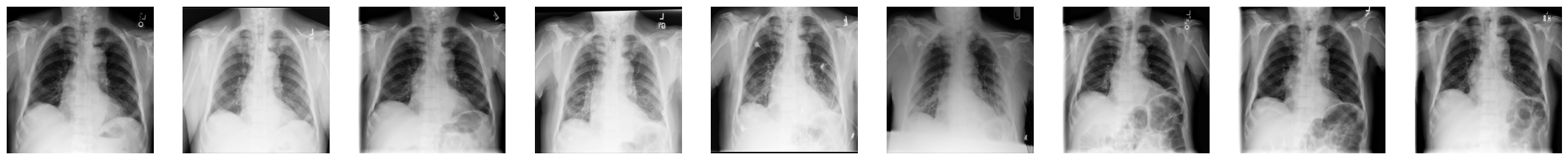
將影像組合成多維陣列以展示進展#
在下一個範例中,您將使用 9 張來自 ChestX-ray8 資料集的 X 光 1024x1024 像素影像,而不是 1 張影像,這些影像已從其中一個資料集檔案中下載和提取。它們的編號從 ...000.png 到 ...008.png,讓我們假設它們屬於同一位患者。
1. 匯入 NumPy,讀取每個 X 光片,並建立一個三維陣列,其中第一個維度對應於影像編號
import numpy as np
num_imgs = 9

combined_xray_images_1 = np.array(
    [imageio.v3.imread(os.path.join(DIR, f"00000011_00{i}.png")) for i in range(num_imgs)]
)
2. 檢查包含 9 個堆疊影像的新 X 光影像陣列的形狀
combined_xray_images_1.shape
(9, 1024, 1024)
請注意,第一個維度中的形狀與 num_imgs 相符,因此 combined_xray_images_1 陣列可以解釋為 2D 影像的堆疊。
3. 您現在可以透過使用 Matplotlib 將每個影格彼此相鄰繪製來顯示「健康進展」
fig, axes = plt.subplots(nrows=1, ncols=num_imgs, figsize=(30, 30))

for img, ax in zip(combined_xray_images_1, axes):
    ax.imshow(img, cmap='gray')
    ax.axis('off')
4. 此外,以動畫形式顯示進展可能會有所幫助。讓我們使用 imageio.mimwrite() 建立 GIF 檔案,並在筆記本中顯示結果
GIF_PATH = os.path.join(DIR, "xray_image.gif")
imageio.mimwrite(GIF_PATH, combined_xray_images_1, format= ".gif", duration=1000)
結果如下: 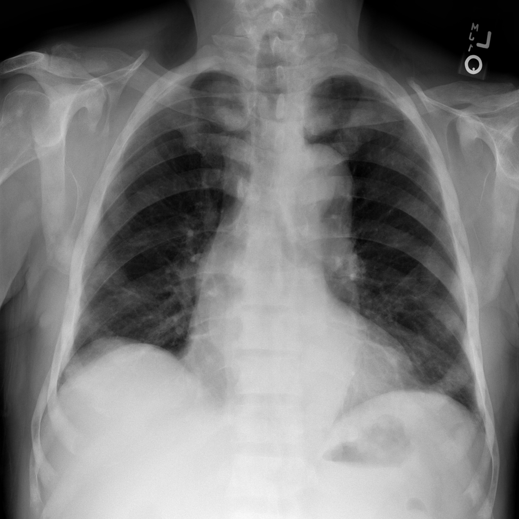
使用 Laplacian-Gaussian、高斯梯度、Sobel 和 Canny 濾波器進行邊緣偵測#
在處理生物醫學資料時,強調 2D 「邊緣」 以聚焦於影像中的特定特徵可能很有用。為此,當偵測顏色像素強度的變化時,使用 影像梯度 可能特別有幫助。
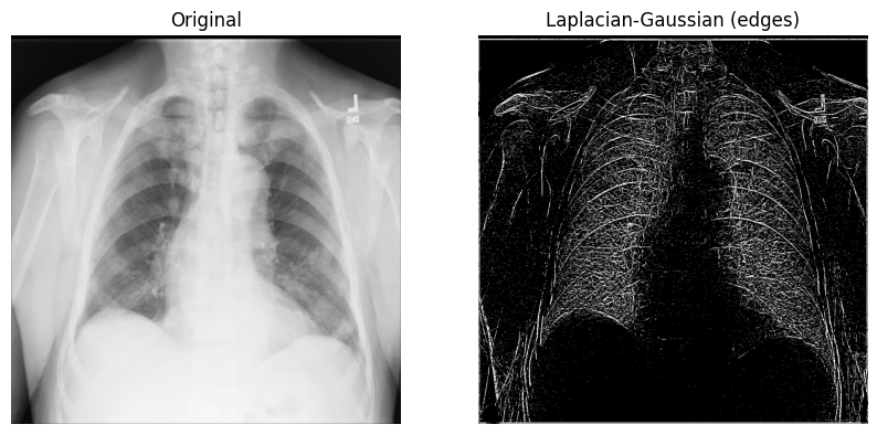
具有高斯二階導數的 Laplace 濾波器#
讓我們從 n 維 Laplace 濾波器(「Laplacian-Gaussian」)開始,它使用 高斯 二階導數。這種拉普拉斯方法專注於像素值強度快速變化的像素,並與高斯平滑相結合以 消除雜訊。讓我們檢查它在分析 2D X 光影像中如何有用。
Laplacian-Gaussian 濾波器的實作相對簡單:1) 從 SciPy 匯入
ndimage模組;以及 2) 使用 sigma(純量)參數呼叫scipy.ndimage.gaussian_laplace(),這會影響高斯濾波器的標準差(在下面的範例中,您將使用1)
from scipy import ndimage

xray_image_laplace_gaussian = ndimage.gaussian_laplace(xray_image, sigma=1)
顯示原始 X 光片和使用 Laplacian-Gaussian 濾波器處理後的 X 光片
fig, axes = plt.subplots(nrows=1, ncols=2, figsize=(10, 10))

axes[0].set_title("Original")
axes[0].imshow(xray_image, cmap="gray")
axes[1].set_title("Laplacian-Gaussian (edges)")
axes[1].imshow(xray_image_laplace_gaussian, cmap="gray")
for i in axes:
    i.axis("off")
plt.show()
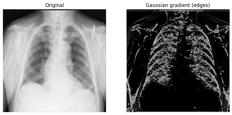
高斯梯度幅度法#
另一種可能有用的邊緣偵測方法是 高斯(梯度)濾波器。它使用高斯導數計算多維梯度幅度,並透過移除 高頻 影像組件來提供幫助。
1. 使用 sigma(純量)參數(用於標準差;在下面的範例中,您將使用 2)呼叫 scipy.ndimage.gaussian_gradient_magnitude()
x_ray_image_gaussian_gradient = ndimage.gaussian_gradient_magnitude(xray_image, sigma=2)
2. 顯示原始 X 光片和使用高斯梯度濾波器處理後的 X 光片
fig, axes = plt.subplots(nrows=1, ncols=2, figsize=(10, 10))

axes[0].set_title("Original")
axes[0].imshow(xray_image, cmap="gray")
axes[1].set_title("Gaussian gradient (edges)")
axes[1].imshow(x_ray_image_gaussian_gradient, cmap="gray")
for i in axes:
    i.axis("off")
plt.show()
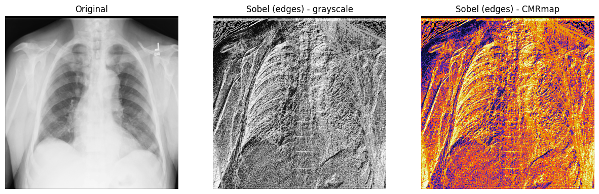
Sobel-Feldman 算子(Sobel 濾波器)#
為了在 2D X 光影像的水平軸和垂直軸上找到高空間頻率區域(邊緣或邊緣圖),您可以使用 Sobel-Feldman 算子(Sobel 濾波器) 技術。 Sobel 濾波器將兩個 3x3 核心矩陣(每個軸一個)透過 卷積 應用到 X 光片上。然後,使用 畢氏定理 組合這兩個點(梯度)以產生梯度幅度。
1. 在 X 光片的 x 軸和 y 軸上使用 Sobel 濾波器 — (scipy.ndimage.sobel())。然後,使用 畢氏定理 和 NumPy 的 np.hypot() 計算 x 和 y(已對其應用 Sobel 濾波器)之間的距離,以獲得幅度。最後,正規化重新縮放的影像,使像素值介於 0 和 255 之間。
影像正規化 遵循 output_channel = 255.0 * (input_channel - min_value) / (max_value - min_value) 公式。因為您使用的是灰階影像,所以只需要正規化一個通道。
x_sobel = ndimage.sobel(xray_image, axis=0)
y_sobel = ndimage.sobel(xray_image, axis=1)

xray_image_sobel = np.hypot(x_sobel, y_sobel)

xray_image_sobel *= 255.0 / np.max(xray_image_sobel)
2. 將新的影像陣列資料類型從 float16 變更為 32 位元浮點格式,以 使其與 Matplotlib 相容
print("The data type - before: ", xray_image_sobel.dtype)

xray_image_sobel = xray_image_sobel.astype("float32")

print("The data type - after: ", xray_image_sobel.dtype)
The data type - before:  float16
The data type - after:  float32
3. 顯示原始 X 光片和應用 Sobel「邊緣」濾波器處理後的 X 光片。請注意,灰階和 CMRmap 色譜都用於幫助強調邊緣
fig, axes = plt.subplots(nrows=1, ncols=3, figsize=(15, 15))

axes[0].set_title("Original")
axes[0].imshow(xray_image, cmap="gray")
axes[1].set_title("Sobel (edges) - grayscale")
axes[1].imshow(xray_image_sobel, cmap="gray")
axes[2].set_title("Sobel (edges) - CMRmap")
axes[2].imshow(xray_image_sobel, cmap="CMRmap")
for i in axes:
    i.axis("off")
plt.show()
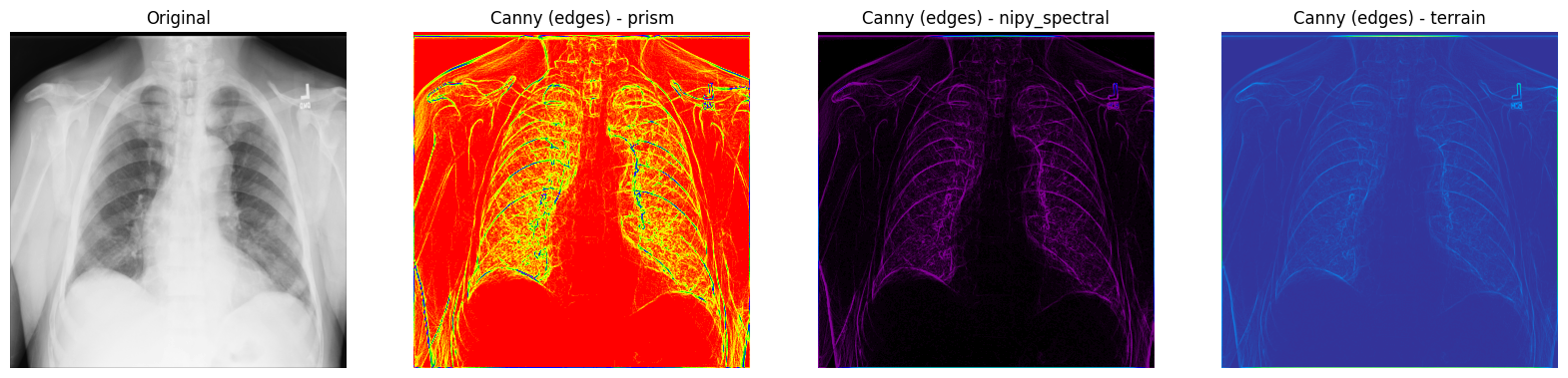
Canny 濾波器#
您也可以考慮使用另一個著名的邊緣偵測濾波器,稱為 Canny 濾波器。
首先,您應用 高斯 濾波器來消除影像中的雜訊。在本範例中,您使用的是 傅立葉 濾波器,它透過 卷積 過程平滑 X 光片。接下來,您在影像的每個 2 個軸上應用 Prewitt 濾波器,以幫助偵測某些邊緣 — 這將產生 2 個梯度值。與 Sobel 濾波器類似,Prewitt 算子也將兩個 3x3 核心矩陣(每個軸一個)透過 卷積 應用到 X 光片上。最後,您使用 畢氏定理 計算兩個梯度之間的幅度,並像之前一樣 正規化 影像。
1. 使用 SciPy 的傅立葉濾波器 — scipy.ndimage.fourier_gaussian() — 和一個小的 sigma 值來消除 X 光片中的一些雜訊。然後,使用 scipy.ndimage.prewitt() 計算兩個梯度。接下來,使用 NumPy 的 np.hypot() 測量梯度之間的距離。最後,像之前一樣 正規化 重新縮放的影像。
fourier_gaussian = ndimage.fourier_gaussian(xray_image, sigma=0.05)

x_prewitt = ndimage.prewitt(fourier_gaussian, axis=0)
y_prewitt = ndimage.prewitt(fourier_gaussian, axis=1)

xray_image_canny = np.hypot(x_prewitt, y_prewitt)

xray_image_canny *= 255.0 / np.max(xray_image_canny)

print("The data type - ", xray_image_canny.dtype)
The data type - float64
2. 繪製原始 X 光影像和使用 Canny 濾波器技術偵測到邊緣的影像。可以使用 prism、nipy_spectral 和 terrain Matplotlib 色譜來強調邊緣。
fig, axes = plt.subplots(nrows=1, ncols=4, figsize=(20, 15))

axes[0].set_title("Original")
axes[0].imshow(xray_image, cmap="gray")
axes[1].set_title("Canny (edges) - prism")
axes[1].imshow(xray_image_canny, cmap="prism")
axes[2].set_title("Canny (edges) - nipy_spectral")
axes[2].imshow(xray_image_canny, cmap="nipy_spectral")
axes[3].set_title("Canny (edges) - terrain")
axes[3].imshow(xray_image_canny, cmap="terrain")
for i in axes:
    i.axis("off")
plt.show()
使用 np.where() 將遮罩應用於 X 光片#
為了篩選出 X 光影像中僅有的某些像素以幫助偵測特定特徵,您可以使用 NumPy 的 np.where(condition: array_like (bool), x: array_like, y: ndarray) 應用遮罩,當 True 時傳回 x,當 False 時傳回 y。
識別感興趣的區域 — 影像中的某些像素集 — 可能很有用,遮罩充當與原始影像形狀相同的布林陣列。
1. 檢索您一直在處理的原始 X 光影像中像素值的一些基本統計資訊
print("The data type of the X-ray image is: ", xray_image.dtype)
print("The minimum pixel value is: ", np.min(xray_image))
print("The maximum pixel value is: ", np.max(xray_image))
print("The average pixel value is: ", np.mean(xray_image))
print("The median pixel value is: ", np.median(xray_image))
The data type of the X-ray image is:  uint8
The minimum pixel value is:  0
The maximum pixel value is:  255
The average pixel value is:  172.52233219146729
The median pixel value is:  195.0
2. 陣列資料類型為 uint8,最小值/最大值結果表明 X 光片中使用了所有 256 種顏色(從 0 到 255)。讓我們使用 ndimage.histogram() 和 Matplotlib 可視化原始原始 X 光影像的像素強度分佈
pixel_intensity_distribution = ndimage.histogram(
    xray_image, min=np.min(xray_image), max=np.max(xray_image), bins=256
)

plt.plot(pixel_intensity_distribution)
plt.title("Pixel intensity distribution")
plt.show()
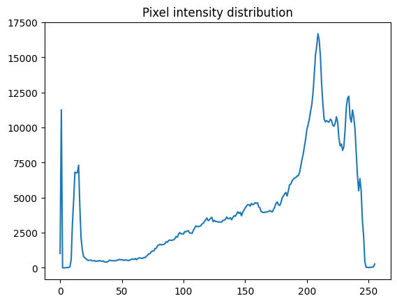
正如像素強度分佈所示,有很多低(大約在 0 到 20 之間)和非常高(大約在 200 到 240 之間)的像素值。
3. 您可以使用 NumPy 的 np.where() 建立不同的條件遮罩 — 例如,讓我們只保留影像中像素值超過特定閾值的值
# The threshold is "greater than 150"
# Return the original image if true, `0` otherwise
xray_image_mask_noisy = np.where(xray_image > 150, xray_image, 0)

plt.imshow(xray_image_mask_noisy, cmap="gray")
plt.axis("off")
plt.show()
# The threshold is "greater than 150"
# Return `1` if true, `0` otherwise
xray_image_mask_less_noisy = np.where(xray_image > 150, 1, 0)

plt.imshow(xray_image_mask_less_noisy, cmap="gray")
plt.axis("off")
plt.show()

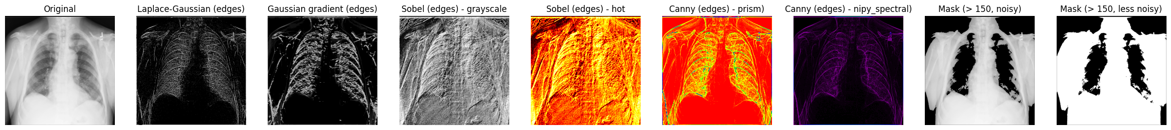
比較結果#
讓我們顯示一些您到目前為止處理過的 X 光影像的結果
fig, axes = plt.subplots(nrows=1, ncols=9, figsize=(30, 30))

axes[0].set_title("Original")
axes[0].imshow(xray_image, cmap="gray")
axes[1].set_title("Laplace-Gaussian (edges)")
axes[1].imshow(xray_image_laplace_gaussian, cmap="gray")
axes[2].set_title("Gaussian gradient (edges)")
axes[2].imshow(x_ray_image_gaussian_gradient, cmap="gray")
axes[3].set_title("Sobel (edges) - grayscale")
axes[3].imshow(xray_image_sobel, cmap="gray")
axes[4].set_title("Sobel (edges) - hot")
axes[4].imshow(xray_image_sobel, cmap="hot")
axes[5].set_title("Canny (edges) - prism)")
axes[5].imshow(xray_image_canny, cmap="prism")
axes[6].set_title("Canny (edges) - nipy_spectral)")
axes[6].imshow(xray_image_canny, cmap="nipy_spectral")
axes[7].set_title("Mask (> 150, noisy)")
axes[7].imshow(xray_image_mask_noisy, cmap="gray")
axes[8].set_title("Mask (> 150, less noisy)")
axes[8].imshow(xray_image_mask_less_noisy, cmap="gray")
for i in axes:
    i.axis("off")
plt.show()
後續步驟#
如果您想使用自己的樣本,可以使用 此影像,或在 Openi 資料庫中搜尋各種其他影像。 Openi 包含許多生物醫學影像,如果您頻寬較低和/或下載資料量受到限制,它可能會特別有幫助。
若要深入了解生物醫學影像資料背景下的影像處理或僅是邊緣偵測,您可能會發現以下材料很有用
使用 Scikit-Image 和 pydicom 進行 Python 中的 DICOM 處理和分割 (Radiology Data Quest)
使用 Numpy 和 Scipy 進行影像操作和處理 (Scipy Lecture Notes)
強度值 (簡報,DataCamp)
使用 Raspberry Pi 和 Python 進行物件偵測 (Maker Portal)
使用深度學習進行 X 光資料準備和分割 (Kaggle 託管的 Jupyter 筆記本)
影像濾波 (演講投影片,CS6670:電腦視覺,康乃爾大學)
Python 和 NumPy 中的邊緣偵測 (Towards Data Science)
使用 Scikit-Image 進行 邊緣偵測 (Data Carpentry)
影像梯度和梯度濾波 (演講投影片,16-385 電腦視覺,卡內基美隆大學)