使用 NumPy 中的真實數據確定摩爾定律#

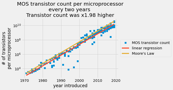
Scatter plot of MOS transistor count per microprocessor every two years as a demonstration of Moore's Law.

在 y 軸上以對數刻度繪製的每個晶片報告的電晶體數量，x 軸上以線性刻度繪製的導入日期。藍色數據點來自電晶體計數表。紅線是普通最小平方法預測，橙線是摩爾定律。

您將做什麼#

1965 年，工程師 Gordon Moore 預測，在接下來的十年中，晶片上的電晶體數量將每兩年翻一番 [1]。您將比較摩爾的預測與他預測後 53 年的實際電晶體數量。您將確定最佳擬合常數，以描述半導體上電晶體的指數成長與摩爾定律的比較。

您將學到的技能#

從 *.csv 檔案載入數據
執行線性迴歸並使用普通最小平方法預測指數成長
您將比較模型之間的指數成長常數
在檔案中分享您的分析
- 以 NumPy 壓縮檔案 *.npz 格式
- 以 *.csv 檔案格式
評估半導體製造商在過去五十年中取得的驚人進展

您需要的東西#

1. 這些套件

NumPy
Matplotlib

使用以下命令導入

import matplotlib.pyplot as plt
import numpy as np

2. 由於這是指數成長定律，您需要一些使用自然對數和指數進行數學運算的背景知識。

您將使用這些 NumPy 和 Matplotlib 函數

np.loadtxt：此函數將文字載入到 NumPy 陣列中
np.log：此函數取得 NumPy 陣列中所有元素的自然對數
np.exp：此函數取得 NumPy 陣列中所有元素的指數
lambda：這是用於建立函數模型的最小函數定義
plt.semilogy：此函數將 x-y 數據繪製到具有線性 x 軸和 $\log_{10}$ y 軸的圖形上 plt.plot：此函數將 x-y 數據繪製在線性軸上
切片陣列：檢視載入到工作區的數據部分，切片陣列，例如 x[:10] 表示陣列中的前 10 個值，x
布林陣列索引：要檢視符合給定條件的數據部分，請使用布林運算來索引陣列
np.block：將陣列組合成 2D 陣列
np.newaxis：將 1D 向量變更為行向量或列向量
np.savez 和 np.savetxt：這兩個函數將分別以壓縮陣列格式和文字格式儲存您的陣列

將摩爾定律建立為指數函數#

您的經驗模型假設每個半導體的電晶體數量都遵循指數成長，

$\log(\text{transistor_count})= f(\text{year}) = A\cdot \text{year}+B,$

其中 $A$ 和 $B$ 是擬合常數。您使用半導體製造商的數據來尋找擬合常數。

您透過指定新增電晶體的速率 2，並為給定年份提供初始電晶體數量，來確定摩爾定律的這些常數。

您以指數形式陳述摩爾定律如下：

$\text{transistor_count}= e^{A_M\cdot \text{year} +B_M}.$

其中 $A_M$ 和 $B_M$ 是常數，它們使電晶體數量每兩年翻一番，並從 1971 年的 2250 個電晶體開始，

$\dfrac{\text{transistor_count}(\text{year} +2)}{\text{transistor_count}(\text{year})} = 2 = \dfrac{e^{B_M}e^{A_M \text{year} + 2A_M}}{e^{B_M}e^{A_M \text{year}}} = e^{2A_M} \rightarrow A_M = \frac{\log(2)}{2}$
$\log(2250) = \frac{\log(2)}{2}\cdot 1971 + B_M \rightarrow B_M = \log(2250)-\frac{\log(2)}{2}\cdot 1971$

因此，以指數函數表示的摩爾定律為

$\log(\text{transistor_count})= A_M\cdot \text{year}+B_M,$

其中

$A_M=0.3466$

$B_M=-675.4$

由於此函數代表摩爾定律，請使用 lambda 將其定義為 Python 函數

A_M = np.log(2) / 2
B_M = np.log(2250) - A_M * 1971
Moores_law = lambda year: np.exp(B_M) * np.exp(A_M * year)

1971 年，Intel 4004 晶片上有 2250 個電晶體。使用 Moores_law 檢查 Gordon Moore 預期 1973 年的半導體數量。

ML_1971 = Moores_law(1971)
ML_1973 = Moores_law(1973)
print("In 1973, G. Moore expects {:.0f} transistors on Intels chips".format(ML_1973))
print("This is x{:.2f} more transistors than 1971".format(ML_1973 / ML_1971))

In 1973, G. Moore expects 4500 transistors on Intels chips
This is x2.00 more transistors than 1971

將歷史製造數據載入到您的工作區#

現在，根據每個晶片的歷史半導體數據做出預測。電晶體計數 [3] 每年都在 transistor_data.csv 檔案中。在將 *.csv 檔案載入到 NumPy 陣列之前，最好先檢查檔案的結構。然後，找到感興趣的列並將其儲存到變數中。將檔案的兩列儲存到陣列 data。

在此，印出 transistor_data.csv 的前 10 列。這些列是

處理器	MOS 電晶體計數	導入日期	設計者	MOSprocess	面積
Intel 4004 (4 位元 16-pin)	2250	1971	Intel	“10,000 nm”	12 mm²
…	…	…	…	…	…

! head transistor_data.csv

Processor,MOS transistor count,Date of Introduction,Designer,MOSprocess,Area
Intel 4004 (4-bit  16-pin),2250,1971,Intel,"10,000 nm",12 mm²
Intel 8008 (8-bit  18-pin),3500,1972,Intel,"10,000 nm",14 mm²
NEC μCOM-4 (4-bit  42-pin),2500,1973,NEC,"7,500 nm",?
Intel 4040 (4-bit  16-pin),3000,1974,Intel,"10,000 nm",12 mm²
Motorola 6800 (8-bit  40-pin),4100,1974,Motorola,"6,000 nm",16 mm²
Intel 8080 (8-bit  40-pin),6000,1974,Intel,"6,000 nm",20 mm²
TMS 1000 (4-bit  28-pin),8000,1974,Texas Instruments,"8,000 nm",11 mm²
MOS Technology 6502 (8-bit  40-pin),4528,1975,MOS Technology,"8,000 nm",21 mm²
Intersil IM6100 (12-bit  40-pin; clone of PDP-8),4000,1975,Intersil,,

您不需要指定處理器、設計者、MOSprocess 或面積的列。剩下第二列和第三列，分別是MOS 電晶體計數和導入日期。

接下來，您使用 np.loadtxt 將這兩列載入到 NumPy 陣列中。以下額外選項會將數據置於所需的格式

delimiter = ','：將分隔符指定為逗號 ‘,’（這是預設行為）
usecols = [1,2]：從 csv 匯入第二列和第三列
skiprows = 1：不要使用第一列，因為它是標題列

data = np.loadtxt("transistor_data.csv", delimiter=",", usecols=[1, 2], skiprows=1)

您已將半導體的整個歷史記錄載入到名為 data 的 NumPy 陣列中。第一列是 MOS 電晶體計數，第二列是以四位數字年份表示的導入日期。

接下來，透過將這兩列分配給變數 year 和 transistor_count，使數據更易於閱讀和管理。透過使用 [:10] 切片 year 和 transistor_count 陣列，印出前 10 個值。印出這些值以檢查您是否已將數據儲存到正確的變數中。

year = data[:, 1]  # grab the second column and assign
transistor_count = data[:, 0]  # grab the first column and assign

print("year:\t\t", year[:10])
print("trans. cnt:\t", transistor_count[:10])

year:		 [1971. 1972. 1973. 1974. 1974. 1974. 1974. 1975. 1975. 1975.]
trans. cnt:	 [2250. 3500. 2500. 3000. 4100. 6000. 8000. 4528. 4000. 5000.]

您正在建立一個預測給定年份電晶體數量的函數。您有一個自變數 year 和一個應變數 transistor_count。將應變數轉換為對數刻度，

$y_i = \log($ transistor_count[i] $),$

產生線性方程式，

$y_i = A\cdot \text{year} +B$.

yi = np.log(transistor_count)

計算電晶體的歷史成長曲線#

您的模型假設 yi 是 year 的函數。現在，找到最佳擬合模型，以最小化 $y_i$ 和 $A\cdot \text{year} +B, $ 之間的差異，如下所示

$\min \sum|y_i - (A\cdot \text{year}_i + B)|^2.$

這個平方誤差總和可以簡潔地表示為陣列，如下所示

$\sum|\mathbf{y}-\mathbf{Z} [A,~B]^T|^2,$

其中 $\mathbf{y}$ 是 1D 陣列中電晶體數量對數的觀測值，而 $\mathbf{Z}=[\text{year}_i^1,~\text{year}_i^0]$ 是 $\text{year}_i$ 在第一列和第二列中的多項式項。透過在 $\mathbf{Z}-$矩陣中建立這組迴歸量，您可以設定普通最小平方法統計模型。

Z 是具有兩個參數的線性模型，即度數為 1 的多項式。因此，我們可以使用 numpy.polynomial.Polynomial 表示該模型，並使用擬合功能來確定模型參數

model = np.polynomial.Polynomial.fit(year, yi, deg=1)

預設情況下，Polynomial.fit 在由自變數（在本例中為 year）確定的域中執行擬合。可以使用 convert 方法恢復未縮放和未移動模型的係數

model = model.convert()
model

\[x \mapsto \text{-666.32640635} + \text{0.34163208}\,x\]

個別參數 $A$ 和 $B$ 是我們線性模型的係數

B, A = model

製造商是否每兩年將電晶體數量翻一番？您有最終公式，

$\dfrac{\text{transistor_count}(\text{year} +2)}{\text{transistor_count}(\text{year})} = xFactor = \dfrac{e^{B}e^{A( \text{year} + 2)}}{e^{B}e^{A \text{year}}} = e^{2A}$

其中電晶體數量的增加為 $xFactor,$ 年數為 2，$A$ 是半對數函數的最佳擬合斜率。

print(f"Rate of semiconductors added on a chip every 2 years: {np.exp(2 * A):.2f}")

Rate of semiconductors added on a chip every 2 years: 1.98

根據您的最小平方迴歸模型，每個晶片的半導體數量每兩年增加 $1.98$ 倍。您有一個模型可以預測每年的半導體數量。現在將您的模型與實際製造報告進行比較。繪製線性迴歸結果和所有電晶體計數。

在此，使用 plt.semilogy 以對數刻度繪製電晶體數量，以線性刻度繪製年份。您已定義三個陣列以獲得最終模型

$y_i = \log(\text{transistor_count}),$

$y_i = A \cdot \text{year} + B,$

和

$\log(\text{transistor_count}) = A\cdot \text{year} + B,$

您的變數 transistor_count、year 和 yi 都具有相同的維度 (179,)。NumPy 陣列需要相同的維度才能繪圖。預測的電晶體數量現在是

$\text{transistor_count}_{\text{predicted}} = e^Be^{A\cdot \text{year}}$.

在下一個圖中，使用 fivethirtyeight 樣式表。樣式表複製 https://fivethirtyeight.com 元素。使用 plt.style.use 變更 matplotlib 樣式。

transistor_count_predicted = np.exp(B) * np.exp(A * year)
transistor_Moores_law = Moores_law(year)
plt.style.use("fivethirtyeight")
plt.semilogy(year, transistor_count, "s", label="MOS transistor count")
plt.semilogy(year, transistor_count_predicted, label="linear regression")


plt.plot(year, transistor_Moores_law, label="Moore's Law")
plt.title(
    "MOS transistor count per microprocessor\n"
    + "every two years \n"
    + "Transistor count was x{:.2f} higher".format(np.exp(A * 2))
)
plt.xlabel("year introduced")
plt.legend(loc="center left", bbox_to_anchor=(1, 0.5))
plt.ylabel("# of transistors\nper microprocessor")

Text(0, 0.5, '# of transistors\nper microprocessor')

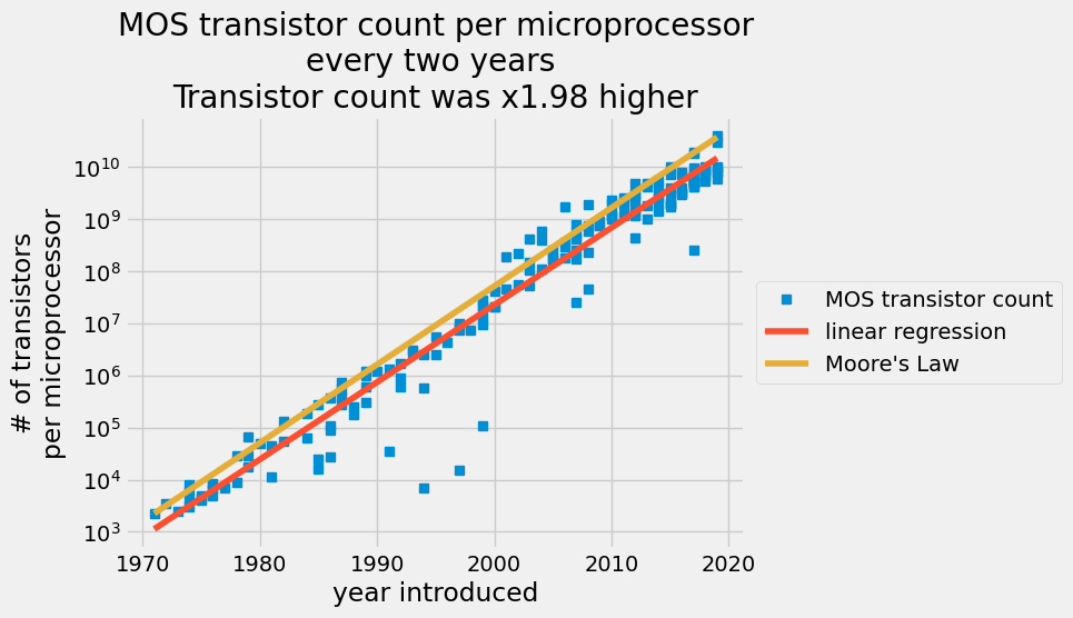
../_images/1144bf4ec876e9f6675dc6c1b67b0fb0638a51e328b5c2fa4ce2d644676acb01.png

每兩年繪製的每個微處理器 MOS 電晶體計數的散佈圖，其中紅線代表普通最小平方法預測，橙線代表摩爾定律。

線性迴歸捕捉了每年每個半導體的電晶體數量的增加。2015 年，半導體製造商聲稱他們無法再跟上摩爾定律。您的分析顯示，自 1971 年以來，電晶體計數的平均增長率為每 2 年 1.98 倍，但 Gordon Moore 預測每 2 年為 2 倍。這是一個驚人的預測。

考慮 2017 年。將數據與您的線性迴歸模型和 Gordon Moore 的預測進行比較。首先，從 2017 年取得電晶體計數。您可以使用布林比較器來執行此操作，

year == 2017.

然後，使用上面定義的 Moores_law 並將您的最佳擬合常數插入到您的函數中，對 2017 年進行預測

$\text{transistor_count} = e^{B}e^{A\cdot \text{year}}$.

比較這些測量值的一個好方法是將您的預測和摩爾的預測與平均電晶體計數進行比較，並查看該年份報告值的範圍。使用 plt.plot 選項 alpha=0.2 以增加數據的透明度。點越不透明，表示測量值上報告的值越多。綠色 $+$ 是 2017 年報告的平均電晶體計數。繪製 $\pm\frac{1}{2}~years 的預測。

transistor_count2017 = transistor_count[year == 2017]
print(
    transistor_count2017.max(), transistor_count2017.min(), transistor_count2017.mean()
)
y = np.linspace(2016.5, 2017.5)
your_model2017 = np.exp(B) * np.exp(A * y)
Moore_Model2017 = Moores_law(y)

plt.plot(
    2017 * np.ones(np.sum(year == 2017)),
    transistor_count2017,
    "ro",
    label="2017",
    alpha=0.2,
)
plt.plot(2017, transistor_count2017.mean(), "g+", markersize=20, mew=6)

plt.plot(y, your_model2017, label="Your prediction")
plt.plot(y, Moore_Model2017, label="Moores law")
plt.ylabel("# of transistors\nper microprocessor")
plt.legend()

19200000000.0 250000000.0 7050000000.0

<matplotlib.legend.Legend at 0x732907357280>

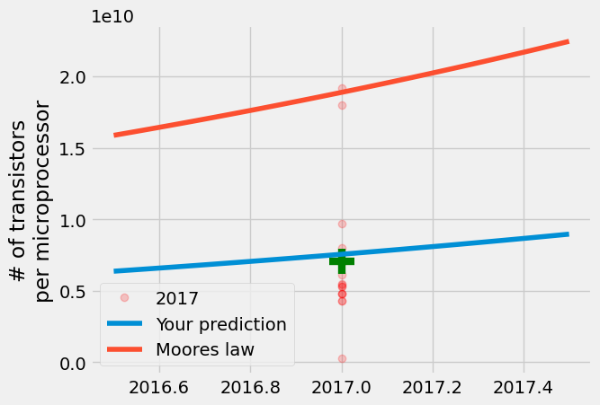
../_images/9914d5c32de9574643975422161b794fad4ff2085c153d60235e0cd8d0f47bff.png

結果是您的模型接近平均值，但 Gordon Moore 的預測更接近 2017 年生產的每個微處理器的最大電晶體數量。即使半導體製造商認為成長會放緩，一次是在 1975 年，現在又接近 2025 年，製造商仍在每 2 年生產半導體，使其電晶體數量幾乎翻一番。

線性迴歸模型更擅長預測平均值而不是極端值，因為它滿足最小化 $\sum |y_i - A\cdot \text{year}[i]+B|^2$ 的條件。

總結#

總之，您已將半導體製造商的歷史數據與摩爾定律進行了比較，並建立了一個線性迴歸模型，以找出每兩年添加到每個微處理器的平均電晶體數量。Gordon Moore 預測從 1965 年到 1975 年，電晶體數量將每兩年翻一番，但從 1971 年到 2019 年，平均成長率一直保持每兩年 $\times 1.98 \pm 0.01$ 的穩定增長。2015 年，摩爾修改了他的預測，表示摩爾定律應持續到 2025 年。[2]。您可以將這些結果作為壓縮的 NumPy 陣列檔案 mooreslaw_regression.npz 或另一個 csv 檔案 mooreslaw_regression.csv 分享。半導體製造的驚人進步推動了新興產業和運算能力。此分析應讓您對過去半個世紀以來的驚人成長略有了解。

使用 NumPy 中的真實數據確定摩爾定律

目錄

使用 NumPy 中的真實數據確定摩爾定律#

您將做什麼#

您將學到的技能#

您需要的東西#

將摩爾定律建立為指數函數#

將歷史製造數據載入到您的工作區#

計算電晶體的歷史成長曲線#

總結#

參考文獻#

使用 NumPy 中的真實數據確定摩爾定律

目錄

使用 NumPy 中的真實數據確定摩爾定律#

您將做什麼#

您將學到的技能#

您需要的東西#

將摩爾定律建立為指數函數#

將歷史製造數據載入到您的工作區#

計算電晶體的歷史成長曲線#

以壓縮陣列和 csv 格式分享您的結果#

將陣列壓縮到檔案中#

建立您自己的逗號分隔值檔案#

總結#

參考文獻#