
過去十年重要演講的情感分析#
注意事項
本文目前尚未經過測試。透過使其完全可執行來協助改進本教學!
本教學示範如何從 NumPy 中從頭開始建構一個簡單的長短期記憶網路 (LSTM),以對具有社會相關性和倫理取得的資料集執行情感分析。
您的深度學習模型 (LSTM) 是一種遞迴神經網路,它將學習從 IMDB 評論資料集中將一段文字分類為正面或負面。該資料集包含 50,000 條電影評論和對應的標籤。基於這些評論的數字表示及其對應的標籤(監督式學習),神經網路將被訓練使用正向傳播和基於時間的反向傳播來學習情感,因為我們這裡處理的是序列數據。輸出將是一個向量,其中包含文字樣本為正面的機率。
如今,深度學習正被應用於日常生活中,現在更重要的是要確保使用 AI 做出的決策不會反映出對特定人群的歧視行為。在使用 AI 輸出時,務必將公平性納入考量。在本教學過程中,我們將嘗試從倫理角度質疑流程中的所有步驟。
先決條件#
你需要熟悉 Python 程式語言以及使用 NumPy 進行陣列操作。此外,建議你對線性代數和微積分有一定的了解。你也應該熟悉神經網路的運作方式。參考資源如下:Python、n 維陣列上的線性代數 以及 微積分 教學。
若要複習深度學習的基礎知識,建議你閱讀 d2l.ai 電子書,這是一本互動式深度學習書籍,包含多框架程式碼、數學和討論。你也可以參考 從零開始在 MNIST 上進行深度學習教學,了解如何從頭實作一個基本的神經網路。
除了 NumPy 之外,你還將使用以下 Python 標準模組來進行資料載入和處理:
使用
pandas處理資料框架使用
Matplotlib進行資料視覺化使用
pooch下載和快取資料集
本教學可以在隔離的環境中本機執行,例如 Virtualenv 或 conda。你可以使用 Jupyter Notebook 或 JupyterLab 來執行每個 notebook 儲存格。
目錄#
資料收集
預處理資料集
從零開始建構和訓練 LSTM 網路
對收集到的演講進行情感分析
後續步驟
1. 資料收集#
在開始之前,有一些重點你應該在選擇用於訓練模型的資料之前牢記在心
識別資料偏差 - 偏差是人類思維過程中固有的組成部分。因此,來自人類活動的資料反映了這種偏差。這種偏差在機器學習資料集中經常出現的一些方式是:
歷史資料中的偏差:歷史資料通常會偏向或不利於特定群體。資料也可能嚴重失衡,關於受保護群體的資訊有限。
資料收集機制中的偏差:缺乏代表性會在資料收集過程中引入固有的偏差。
對可觀察結果的偏差:在某些情況下,我們只掌握了特定人群的真實結果資訊。在缺乏所有結果資訊的情況下,人們甚至無法衡量公平性。
保護敏感資料中的人類匿名性:Trevisan 和 Reilly 列出了一系列需要格外小心處理的敏感主題。我們將其列示如下,並添加了一些補充:
個人日常生活(包含位置數據);
個人損傷和/或醫療記錄的詳細資訊;
關於疼痛和慢性疾病的情緒描述;
關於收入和/或福利金的財務資訊;
歧視和虐待事件;
對個別醫療保健和支持服務提供者的批評/讚揚;
自殺念頭;
對權力結構的批評/讚揚,尤其是在危及自身安全的情況下;
個人身份資訊(即使以某種方式匿名化),包含指紋或聲音等。
雖然從這麼多人身上取得同意可能很困難,尤其是在線上平台上,但其必要性取決於你的數據包含的主題的敏感性,以及其他指標,例如數據來源平台是否允許用戶使用假名操作。如果網站的政策強制使用真實姓名,則需要徵求用戶的同意。
在本節中,你將收集兩個不同的數據集:IMDb 電影評論數據集,以及為本教學課程策劃的 10 篇演講集,其中包含來自世界各地不同國家、不同時代和不同主題的行動主義者的演講。前者將用於訓練深度學習模型,而後者將用於執行情感分析。
收集 IMDb 評論數據集#
IMDb 評論數據集是一個大型電影評論數據集,由 Andrew L. Maas 從熱門電影評分服務 IMDb 收集和準備。IMDb 評論數據集用於二元情感分類,即評論是正面還是負面。它包含 25,000 條電影評論用於訓練,25,000 條用於測試。所有這 50,000 條評論都是標記數據,可用於監督式深度學習。為了便於重現性,我們將從 Zenodo 獲取數據。
IMDb 平台允許將其公開數據集用於個人和非商業用途。我們已盡最大努力確保這些評論不包含任何上述與評論者相關的敏感主題。
收集並載入演講稿#
我們選擇了全球各地行動主義者的演講,他們談論氣候變遷、女性主義、LGBTQA+ 權利和種族主義等議題。這些演講來自報紙、聯合國官方網站和知名大學的檔案,如下表所示。我們創建了一個 CSV 檔案,其中包含演講稿、演講者以及演講來源。我們確保在數據中包含不同的人口統計資料,並涵蓋各種不同的主題,其中大部分關注社會和/或倫理議題。
2. 資料預處理#
在建立任何深度學習模型之前,資料預處理都是至關重要的步驟。然而,為了讓本教學專注於模型的建構,我們不會深入探討預處理的程式碼。以下簡要概述我們清理資料並將其轉換為數值表示形式的所有步驟。
文字去噪:在將文字轉換為向量之前,務必先清理並移除所有無用的部分,也就是資料中的雜訊。這可以透過將所有字元轉換為小寫、移除 HTML 標籤、括號和停用詞(對句子沒有太多意義的詞)來完成。如果沒有這個步驟,資料集通常會是一堆電腦無法理解的詞彙。
將文字轉換為向量:詞嵌入是一種文字的學習表示法,其中具有相同含義的詞具有相似的表示形式。每個詞彙在預定義的向量空間中表示為實值向量。GloVe 是由史丹佛大學開發的一種非監督式演算法,用於透過從語料庫生成全局詞彙共現矩陣來生成詞嵌入。您可以從 https://nlp.stanford.edu/projects/glove/ 下載包含嵌入的壓縮檔。在此,您可以從四個選項中選擇不同大小或訓練資料集的檔案。我們選擇了記憶體消耗最少的嵌入檔。
GloVe 詞嵌入包含在數十億個詞彙上訓練的集合,有些甚至高達 8400 億個詞彙。這些演算法會呈現刻板印象的偏差,例如性別偏差,這可以追溯到原始訓練資料。例如,某些職業似乎更偏向特定性別,強化了有問題的刻板印象。解決此問題的最近似方法是一些去偏差演算法,例如 https://web.stanford.edu/class/archive/cs/cs224n/cs224n.1184/reports/6835575.pdf 中提出的演算法,可以用於您選擇的嵌入以減輕偏差(如果有的話)。
您將從導入構建深度學習網路所需的套件開始。
# Importing the necessary packages
import numpy as np
import pandas as pd
import matplotlib.pyplot as plt
import pooch
import string
import re
import zipfile
import os

# Creating the random instance
rng = np.random.default_rng()
接下來,您將定義一組文字預處理輔助函式。
class TextPreprocess:
    """Text Preprocessing for a Natural Language Processing model."""

    def txt_to_df(self, file):
        """Function to convert a txt file to pandas dataframe.

        Parameters
        ----------
        file : str
            Path to the txt file.

        Returns
        -------
        Pandas dataframe
            txt file converted to a dataframe.

        """
        with open(imdb_train, 'r') as in_file:
            stripped = (line.strip() for line in in_file)
            reviews = {}
            for line in stripped:
                lines = [splits for splits in line.split("\t") if splits != ""]
                reviews[lines[1]] = float(lines[0])
        df = pd.DataFrame(reviews.items(), columns=['review', 'sentiment'])
        df = df.sample(frac=1).reset_index(drop=True)
        return df

    def unzipper(self, zipped, to_extract):
        """Function to extract a file from a zipped folder.

        Parameters
        ----------
        zipped : str
            Path to the zipped folder.

        to_extract: str
            Path to the file to be extracted from the zipped folder

        Returns
        -------
        str
            Path to the extracted file.

        """
        fh = open(zipped, 'rb')
        z = zipfile.ZipFile(fh)
        outdir = os.path.split(zipped)[0]
        z.extract(to_extract, outdir)
        fh.close()
        output_file = os.path.join(outdir, to_extract)
        return output_file

    def cleantext(self, df, text_column=None,
                  remove_stopwords=True, remove_punc=True):
        """Function to clean text data.

        Parameters
        ----------
        df : pandas dataframe
            The dataframe housing the input data.
        text_column : str
            Column in dataframe whose text is to be cleaned.
        remove_stopwords : bool
            if True, remove stopwords from text
        remove_punc : bool
            if True, remove punctuation symbols from text

        Returns
        -------
        Numpy array
            Cleaned text.

        """
        # converting all characters to lowercase
        df[text_column] = df[text_column].str.lower()

        # List of stopwords taken from https://gist.github.com/sebleier/554280
        stopwords = ["a", "about", "above", "after", "again", "against",
                     "all", "am", "an", "and", "any", "are",
                     "as", "at", "be", "because",
                     "been", "before", "being", "below",
                     "between", "both", "but", "by", "could",
                     "did", "do", "does", "doing", "down", "during",
                     "each", "few", "for", "from", "further",
                     "had", "has", "have", "having", "he",
                     "he'd", "he'll", "he's", "her", "here",
                     "here's", "hers", "herself", "him",
                     "himself", "his", "how", "how's", "i",
                     "i'd", "i'll", "i'm", "i've",
                     "if", "in", "into",
                     "is", "it", "it's", "its",
                     "itself", "let's", "me", "more",
                     "most", "my", "myself", "nor", "of",
                     "on", "once", "only", "or",
                     "other", "ought", "our", "ours",
                     "ourselves", "out", "over", "own", "same",
                     "she", "she'd", "she'll", "she's", "should",
                     "so", "some", "such", "than", "that",
                     "that's", "the", "their", "theirs", "them",
                     "themselves", "then", "there", "there's",
                     "these", "they", "they'd", "they'll",
                     "they're", "they've", "this", "those",
                     "through", "to", "too", "under", "until", "up",
                     "very", "was", "we", "we'd", "we'll",
                     "we're", "we've", "were", "what",
                     "what's", "when", "when's",
                     "where", "where's",
                     "which", "while", "who", "who's",
                     "whom", "why", "why's", "with",
                     "would", "you", "you'd", "you'll",
                     "you're", "you've",
                     "your", "yours", "yourself", "yourselves"]

        def remove_stopwords(data, column):
            data[f'{column} without stopwords'] = data[column].apply(
                lambda x: ' '.join([word for word in x.split() if word not in (stopwords)]))
            return data

        def remove_tags(string):
            result = re.sub('<*>', '', string)
            return result

        # remove html tags and brackets from text
        if remove_stopwords:
            data_without_stopwords = remove_stopwords(df, text_column)
            data_without_stopwords[f'clean_{text_column}'] = data_without_stopwords[f'{text_column} without stopwords'].apply(
                lambda cw: remove_tags(cw))
        if remove_punc:
            data_without_stopwords[f'clean_{text_column}'] = data_without_stopwords[f'clean_{text_column}'].str.replace(
                '[{}]'.format(string.punctuation), ' ', regex=True)

        X = data_without_stopwords[f'clean_{text_column}'].to_numpy()

        return X


    def sent_tokeniser(self, x):
        """Function to split text into sentences.

        Parameters
        ----------
        x : str
            piece of text

        Returns
        -------
        list
            sentences with punctuation removed.

        """
        sentences = re.split(r'(?<!\w\.\w.)(?<![A-Z][a-z]\.)(?<=\.|\?)\s', x)
        sentences.pop()
        sentences_cleaned = [re.sub(r'[^\w\s]', '', x) for x in sentences]
        return sentences_cleaned

    def word_tokeniser(self, text):
        """Function to split text into tokens.

        Parameters
        ----------
        x : str
            piece of text

        Returns
        -------
        list
            words with punctuation removed.

        """
        tokens = re.split(r"([-\s.,;!?])+", text)
        words = [x for x in tokens if (
            x not in '- \t\n.,;!?\\' and '\\' not in x)]
        return words

    def loadGloveModel(self, emb_path):
        """Function to read from the word embedding file.

        Returns
        -------
        Dict
            mapping from word to corresponding word embedding.

        """
        print("Loading Glove Model")
        File = emb_path
        f = open(File, 'r')
        gloveModel = {}
        for line in f:
            splitLines = line.split()
            word = splitLines[0]
            wordEmbedding = np.array([float(value) for value in splitLines[1:]])
            gloveModel[word] = wordEmbedding
        print(len(gloveModel), " words loaded!")
        return gloveModel

    def text_to_paras(self, text, para_len):
        """Function to split text into paragraphs.

        Parameters
        ----------
        text : str
            piece of text

        para_len : int
            length of each paragraph

        Returns
        -------
        list
            paragraphs of specified length.

        """
        # split the speech into a list of words
        words = text.split()
        # obtain the total number of paragraphs
        no_paras = int(np.ceil(len(words)/para_len))
        # split the speech into a list of sentences
        sentences = self.sent_tokeniser(text)
        # aggregate the sentences into paragraphs
        k, m = divmod(len(sentences), no_paras)
        agg_sentences = [sentences[i*k+min(i, m):(i+1)*k+min(i+1, m)] for i in range(no_paras)]
        paras = np.array([' '.join(sents) for sents in agg_sentences])

        return paras
Pooch 是一個由科學家製作的 Python 套件,用於管理透過 HTTP 下載資料檔案並將其儲存在本機目錄中。我們使用它來設定一個下載管理器,其中包含擷取我們註冊表中的資料檔案並將其儲存在指定快取資料夾中所需的所有資訊。
data = pooch.create(
    # folder where the data will be stored in the
    # default cache folder of your Operating System
    path=pooch.os_cache("numpy-nlp-tutorial"),
    # Base URL of the remote data store
    base_url="",
    # The cache file registry. A dictionary with all files managed by this pooch.
    # The keys are the file names and values are their respective hash codes which
    # ensure we download the same, uncorrupted file each time.
    registry={
        "imdb_train.txt": "6a38ea6ab5e1902cc03f6b9294ceea5e8ab985af991f35bcabd301a08ea5b3f0",
         "imdb_test.txt": "7363ef08ad996bf4233b115008d6d7f9814b7cc0f4d13ab570b938701eadefeb",
        "glove.6B.50d.zip": "617afb2fe6cbd085c235baf7a465b96f4112bd7f7ccb2b2cbd649fed9cbcf2fb",
    },
    # Now specify custom URLs for some of the files in the registry.
    urls={
        "imdb_train.txt": "doi:10.5281/zenodo.4117827/imdb_train.txt",
        "imdb_test.txt": "doi:10.5281/zenodo.4117827/imdb_test.txt",
        "glove.6B.50d.zip": 'https://nlp.stanford.edu/data/glove.6B.zip'
    }
)
下載 IMDb 訓練和測試資料檔案
imdb_train = data.fetch('imdb_train.txt')
imdb_test = data.fetch('imdb_test.txt')
實例化 TextPreprocess 類別以對我們的資料集執行各種操作
textproc = TextPreprocess()
將每個 IMDb 檔案轉換為 pandas 資料框架,以便更方便地預處理資料集
train_df = textproc.txt_to_df(imdb_train)
test_df = textproc.txt_to_df(imdb_test)
現在,您將透過移除停用詞和標點符號來清理上面獲得的資料框架。您還將從每個資料框架中擷取情感值以獲得目標變數
X_train = textproc.cleantext(train_df,
                       text_column='review',
                       remove_stopwords=True,
                       remove_punc=True)[0:2000]

X_test = textproc.cleantext(test_df,
                       text_column='review',
                       remove_stopwords=True,
                       remove_punc=True)[0:1000]

y_train = train_df['sentiment'].to_numpy()[0:2000]
y_test = test_df['sentiment'].to_numpy()[0:1000]
相同的流程適用於收集的演講
由於我們將在教學的後續部分對每個演講進行段落情感分析,因此我們需要標點符號來將文字分成段落,因此我們在此階段不移除標點符號
speech_data_path = 'tutorial-nlp-from-scratch/speeches.csv'
speech_df = pd.read_csv(speech_data_path)
X_pred = textproc.cleantext(speech_df,
                            text_column='speech',
                            remove_stopwords=True,
                            remove_punc=False)
speakers = speech_df['speaker'].to_numpy()
您現在將下載 GloVe 嵌入、解壓縮它們,並建立一個將每個詞彙和詞彙嵌入對應的字典。這將在您需要用各自的詞嵌入替換每個詞彙時充當快取。
glove = data.fetch('glove.6B.50d.zip')
emb_path = textproc.unzipper(glove, 'glove.6B.300d.txt')
emb_matrix = textproc.loadGloveModel(emb_path)
3. 建立深度學習模型#
現在是開始實作我們的 LSTM 的時候了!您必須先熟悉深度學習模型基本建構塊的一些高階概念。您可以參考 從零開始在 MNIST 上進行深度學習的教學。
接下來,您將學習遞迴神經網路 (RNN) 與一般神經網路的區別,以及它為何如此適合處理序列數據。之後,您將使用 Python 和 NumPy 構建一個簡單的深度學習模型,並訓練它學習以一定的準確度將文本的情感分類為正面或負面。
長短期記憶網路簡介#
在多層感知器 (MLP) 中,資訊只朝一個方向移動——從輸入層,經過隱藏層,到輸出層。資訊直接通過網路,且在後續階段絕不會考慮先前的節點。由於它只考慮當前的輸入,學習到的特徵不會在序列的不同位置共享。此外,它無法處理長度不同的序列。
與 MLP 不同,RNN 的設計目的是處理序列預測問題。RNN 引入狀態變數來儲存過去的資訊,並結合當前的輸入來決定當前的輸出。由於 RNN 與序列中的所有數據點共享學習到的特徵,而不管其長度如何,因此它能夠處理長度不同的序列。
然而,RNN 的問題在於它無法保留長期記憶,因為給定輸入對隱藏層的影響,以及因此對網路輸出的影響,會隨著它在網路的遞迴連接中循環而呈指數級衰減或爆炸。這個缺點被稱為梯度消失問題。長短期記憶 (LSTM) 是一種專門設計用於解決梯度消失問題的 RNN 架構。
模型架構概述#
在上面的 gif 中,標記為 \(A\) 的矩形稱為 細胞,它們是 LSTM 網路的**記憶區塊**。它們負責選擇在序列中記住的內容,並通過兩個稱為 隱藏狀態 \(H_{t}\) 和 細胞狀態 \(C_{t}\) 的狀態將這些資訊傳遞給下一個細胞,其中 \(t\) 表示時間步長。每個 細胞 都有專用的閘門,負責儲存、寫入或讀取傳遞給 LSTM 的資訊。您現在將透過實作其中發生的每個機制來仔細研究網路的架構。
讓我們從編寫一個函式開始,隨機初始化模型訓練時將學習的參數。
def initialise_params(hidden_dim, input_dim):
    # forget gate
    Wf = rng.standard_normal(size=(hidden_dim, hidden_dim + input_dim))
    bf = rng.standard_normal(size=(hidden_dim, 1))
    # input gate
    Wi = rng.standard_normal(size=(hidden_dim, hidden_dim + input_dim))
    bi = rng.standard_normal(size=(hidden_dim, 1))
    # candidate memory gate
    Wcm = rng.standard_normal(size=(hidden_dim, hidden_dim + input_dim))
    bcm = rng.standard_normal(size=(hidden_dim, 1))
    # output gate
    Wo = rng.standard_normal(size=(hidden_dim, hidden_dim + input_dim))
    bo = rng.standard_normal(size=(hidden_dim, 1))

    # fully connected layer for classification
    W2 = rng.standard_normal(size=(1, hidden_dim))
    b2 = np.zeros((1, 1))

    parameters = {
        "Wf": Wf,
        "bf": bf,
        "Wi": Wi,
        "bi": bi,
        "Wcm": Wcm,
        "bcm": bcm,
        "Wo": Wo,
        "bo": bo,
        "W2": W2,
        "b2": b2
    }
    return parameters
正向傳播#
現在您已經初始化了參數,您可以將輸入數據沿正向方向傳遞通過網路。每一層都接受輸入數據,處理它,並將其傳遞給下一層。這個過程稱為 正向傳播。您將執行以下機制來實作它:
載入輸入數據的詞嵌入。
將嵌入傳遞給 LSTM。
在 LSTM 的每個記憶區塊中執行所有閘門機制,以獲得最終的隱藏狀態。
將最終的隱藏狀態通過一個全連接層,以獲得序列為正面的機率。
將所有計算出的值儲存在快取中,以便在反向傳播期間使用。
Sigmoid 函數屬於非線性激活函數家族的一員。它幫助網路更新或遺忘數據。如果一個值的 Sigmoid 結果為 0,則該資訊被視為遺忘。同樣地,如果結果為 1,則資訊被保留。
def sigmoid(x):
    n = np.exp(np.fmin(x, 0))
    d = (1 + np.exp(-np.abs(x)))
    return n / d
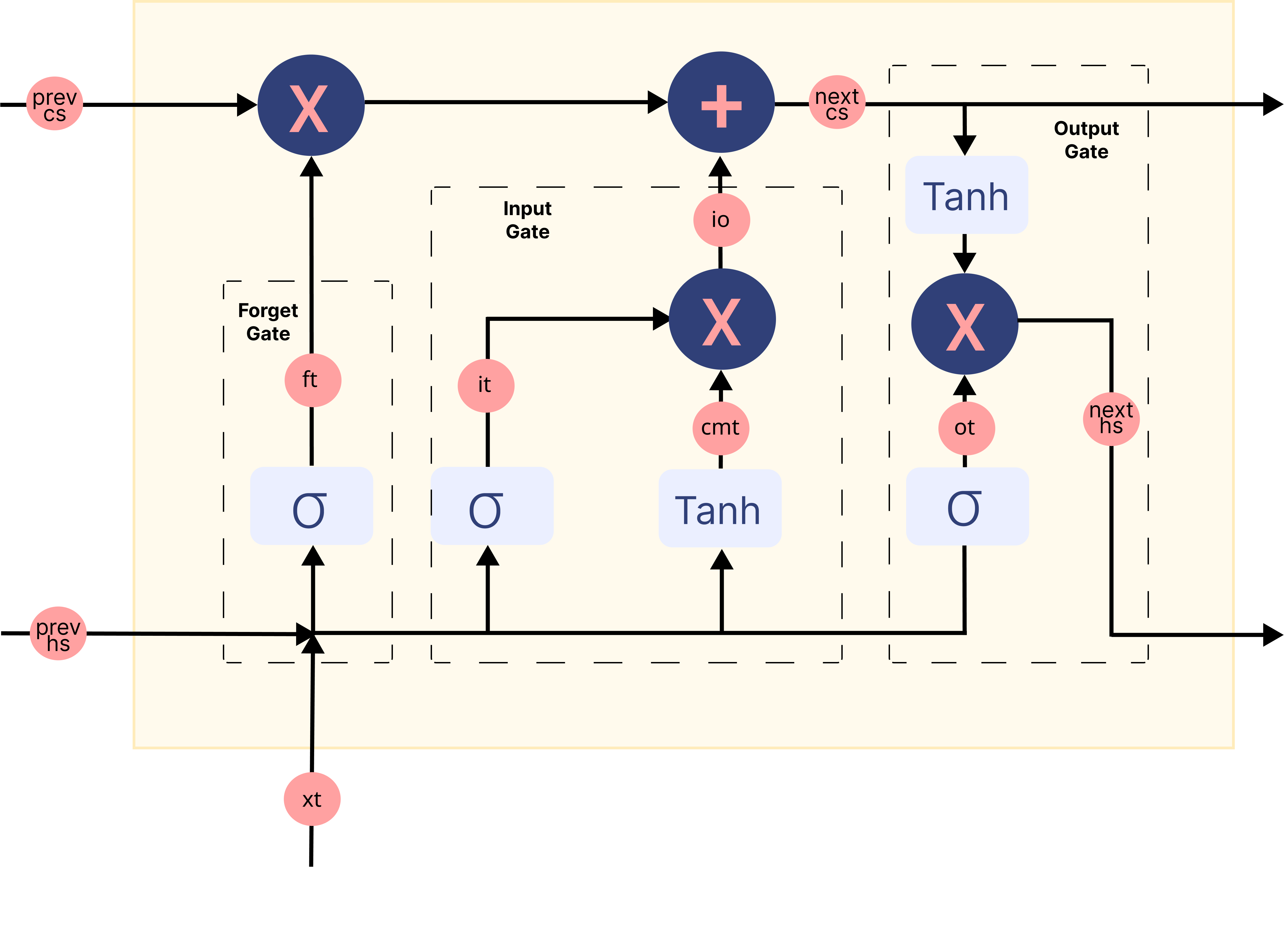
**遺忘門**將目前的詞嵌入和前一個隱藏狀態連接在一起作為輸入,並決定舊記憶單元內容的哪些部分需要關注,哪些可以忽略。
def fp_forget_gate(concat, parameters):
    ft = sigmoid(np.dot(parameters['Wf'], concat)
                 + parameters['bf'])
    return ft
**輸入門**將目前的詞嵌入和前一個隱藏狀態連接在一起作為輸入,並通過**候選記憶門**控制我們考慮多少新數據,而候選記憶門利用 Tanh 函數 來調節流經網路的值。
def fp_input_gate(concat, parameters):
    it = sigmoid(np.dot(parameters['Wi'], concat)
                 + parameters['bi'])
    cmt = np.tanh(np.dot(parameters['Wcm'], concat)
                  + parameters['bcm'])
    return it, cmt
最後,我們有**輸出門**,它接收來自目前詞嵌入、前一個隱藏狀態和已由遺忘門和輸入門更新資訊的單元狀態的資訊,以更新隱藏狀態的值。
def fp_output_gate(concat, next_cs, parameters):
    ot = sigmoid(np.dot(parameters['Wo'], concat)
                 + parameters['bo'])
    next_hs = ot * np.tanh(next_cs)
    return ot, next_hs
下圖總結了 LSTM 網路記憶區塊中的每個門機制
圖片修改自 此 來源
但是如何從 LSTM 的輸出中獲得情感?#
從序列中最後一個記憶區塊的輸出門獲得的隱藏狀態被認為是序列中所有資訊的表示。為了將這些資訊分類到不同的類別(在我們的例子中是 2 個,正面和負面),我們使用**全連接層**,它首先將這些資訊映射到預定義的輸出大小(在我們的例子中是 1)。然後,像是 Sigmoid 這樣的激活函數將此輸出轉換為 0 到 1 之間的值。我們將大於 0.5 的值視為正面情感的指標。
def fp_fc_layer(last_hs, parameters):
    z2 = (np.dot(parameters['W2'], last_hs)
          + parameters['b2'])
    a2 = sigmoid(z2)
    return a2
現在,您將把所有這些函數放在一起,以總結我們模型架構中的**正向傳播**步驟
def forward_prop(X_vec, parameters, input_dim):

    hidden_dim = parameters['Wf'].shape[0]
    time_steps = len(X_vec)

    # Initialise hidden and cell state before passing to first time step
    prev_hs = np.zeros((hidden_dim, 1))
    prev_cs = np.zeros(prev_hs.shape)

    # Store all the intermediate and final values here
    caches = {'lstm_values': [], 'fc_values': []}

    # Hidden state from the last cell in the LSTM layer is calculated.
    for t in range(time_steps):
        # Retrieve word corresponding to current time step
        x = X_vec[t]
        # Retrieve the embedding for the word and reshape it to make the LSTM happy
        xt = emb_matrix.get(x, rng.random(size=(input_dim, 1)))
        xt = xt.reshape((input_dim, 1))

        # Input to the gates is concatenated previous hidden state and current word embedding
        concat = np.vstack((prev_hs, xt))

        # Calculate output of the forget gate
        ft = fp_forget_gate(concat, parameters)

        # Calculate output of the input gate
        it, cmt = fp_input_gate(concat, parameters)
        io = it * cmt

        # Update the cell state
        next_cs = (ft * prev_cs) + io

        # Calculate output of the output gate
        ot, next_hs = fp_output_gate(concat, next_cs, parameters)

        # store all the values used and calculated by
        # the LSTM in a cache for backward propagation.
        lstm_cache = {
        "next_hs": next_hs,
        "next_cs": next_cs,
        "prev_hs": prev_hs,
        "prev_cs": prev_cs,
        "ft": ft,
        "it" : it,
        "cmt": cmt,
        "ot": ot,
        "xt": xt,
        }
        caches['lstm_values'].append(lstm_cache)

        # Pass the updated hidden state and cell state to the next time step
        prev_hs = next_hs
        prev_cs = next_cs

    # Pass the LSTM output through a fully connected layer to
    # obtain probability of the sequence being positive
    a2 = fp_fc_layer(next_hs, parameters)

    # store all the values used and calculated by the
    # fully connected layer in a cache for backward propagation.
    fc_cache = {
    "a2" : a2,
    "W2" : parameters['W2']
    }
    caches['fc_values'].append(fc_cache)
    return caches
反向傳播#
在每次正向傳遞網路後,您將實作 `backpropagation through time` 演算法,以累積每個參數在時間步長上的梯度。由於 LSTM 底層各層相互作用的特殊方式,通過 LSTM 的反向傳播不像通過其他常見深度學習架構那樣簡單。儘管如此,方法大致相同;識別依賴關係並應用鏈式法則。
讓我們從定義一個函數開始,將每個參數的梯度初始化為由與相應參數相同維度的零組成的陣列
# Initialise the gradients
def initialize_grads(parameters):
    grads = {}
    for param in parameters.keys():
        grads[f'd{param}'] = np.zeros((parameters[param].shape))
    return grads
現在,對於每個門和全連接層,我們定義一個函數來計算損失相對於傳遞的輸入和使用的參數的梯度。要了解導數計算背後的數學原理,我們建議您參考 Christina Kouridi 的這篇很有幫助的 部落格文章。
定義一個函數來計算**遺忘門**中的梯度
def bp_forget_gate(hidden_dim, concat, dh_prev, dc_prev, cache, gradients, parameters):
    # dft = dL/da2 * da2/dZ2 * dZ2/dh_prev * dh_prev/dc_prev * dc_prev/dft
    dft = ((dc_prev * cache["prev_cs"] + cache["ot"]
           * (1 - np.square(np.tanh(cache["next_cs"])))
           * cache["prev_cs"] * dh_prev) * cache["ft"] * (1 - cache["ft"]))
    # dWf = dft * dft/dWf
    gradients['dWf'] += np.dot(dft, concat.T)
    # dbf = dft * dft/dbf
    gradients['dbf'] += np.sum(dft, axis=1, keepdims=True)
    # dh_f = dft * dft/dh_prev
    dh_f = np.dot(parameters["Wf"][:, :hidden_dim].T, dft)
    return dh_f, gradients
定義一個函數來計算**輸入門**和**候選記憶門**中的梯度
def bp_input_gate(hidden_dim, concat, dh_prev, dc_prev, cache, gradients, parameters):
    # dit = dL/da2 * da2/dZ2 * dZ2/dh_prev * dh_prev/dc_prev * dc_prev/dit
    dit = ((dc_prev * cache["cmt"] + cache["ot"]
           * (1 - np.square(np.tanh(cache["next_cs"])))
           * cache["cmt"] * dh_prev) * cache["it"] * (1 - cache["it"]))
    # dcmt = dL/da2 * da2/dZ2 * dZ2/dh_prev * dh_prev/dc_prev * dc_prev/dcmt
    dcmt = ((dc_prev * cache["it"] + cache["ot"]
            * (1 - np.square(np.tanh(cache["next_cs"])))
            * cache["it"] * dh_prev) * (1 - np.square(cache["cmt"])))
    # dWi = dit * dit/dWi
    gradients['dWi'] += np.dot(dit, concat.T)
    # dWcm = dcmt * dcmt/dWcm
    gradients['dWcm'] += np.dot(dcmt, concat.T)
    # dbi = dit * dit/dbi
    gradients['dbi'] += np.sum(dit, axis=1, keepdims=True)
    # dWcm = dcmt * dcmt/dbcm
    gradients['dbcm'] += np.sum(dcmt, axis=1, keepdims=True)
    # dhi = dit * dit/dh_prev
    dh_i = np.dot(parameters["Wi"][:, :hidden_dim].T, dit)
    # dhcm = dcmt * dcmt/dh_prev
    dh_cm = np.dot(parameters["Wcm"][:, :hidden_dim].T, dcmt)
    return dh_i, dh_cm, gradients
定義一個函數來計算**輸出門**的梯度
def bp_output_gate(hidden_dim, concat, dh_prev, dc_prev, cache, gradients, parameters):
    # dot = dL/da2 * da2/dZ2 * dZ2/dh_prev * dh_prev/dot
    dot = (dh_prev * np.tanh(cache["next_cs"])
           * cache["ot"] * (1 - cache["ot"]))
    # dWo = dot * dot/dWo
    gradients['dWo'] += np.dot(dot, concat.T)
    # dbo = dot * dot/dbo
    gradients['dbo'] += np.sum(dot, axis=1, keepdims=True)
    # dho = dot * dot/dho
    dh_o = np.dot(parameters["Wo"][:, :hidden_dim].T, dot)
    return dh_o, gradients
定義一個函式來計算**全連接層 (Fully Connected Layer)** 的梯度。
def bp_fc_layer (target, caches, gradients):
    # dZ2 = dL/da2 * da2/dZ2
    predicted = np.array(caches['fc_values'][0]['a2'])
    target = np.array(target)
    dZ2 = predicted - target
    # dW2 = dL/da2 * da2/dZ2 * dZ2/dW2
    last_hs = caches['lstm_values'][-1]["next_hs"]
    gradients['dW2'] = np.dot(dZ2, last_hs.T)
    # db2 = dL/da2 * da2/dZ2 * dZ2/db2
    gradients['db2'] = np.sum(dZ2)
    # dh_last = dZ2 * W2
    W2 = caches['fc_values'][0]["W2"]
    dh_last = np.dot(W2.T, dZ2)
    return dh_last, gradients
將所有這些函式組合在一起,以總結我們模型的**反向傳播 (Backpropagation)** 步驟。
def backprop(y, caches, hidden_dim, input_dim, time_steps, parameters):

    # Initialize gradients
    gradients = initialize_grads(parameters)

    # Calculate gradients for the fully connected layer
    dh_last, gradients = bp_fc_layer(target, caches, gradients)

    # Initialize gradients w.r.t previous hidden state and previous cell state
    dh_prev = dh_last
    dc_prev = np.zeros((dh_prev.shape))

    # loop back over the whole sequence
    for t in reversed(range(time_steps)):
        cache = caches['lstm_values'][t]

        # Input to the gates is concatenated previous hidden state and current word embedding
        concat = np.concatenate((cache["prev_hs"], cache["xt"]), axis=0)

        # Compute gates related derivatives
        # Calculate derivative w.r.t the input and parameters of forget gate
        dh_f, gradients = bp_forget_gate(hidden_dim, concat, dh_prev, dc_prev, cache, gradients, parameters)

        # Calculate derivative w.r.t the input and parameters of input gate
        dh_i, dh_cm, gradients = bp_input_gate(hidden_dim, concat, dh_prev, dc_prev, cache, gradients, parameters)

        # Calculate derivative w.r.t the input and parameters of output gate
        dh_o, gradients = bp_output_gate(hidden_dim, concat, dh_prev, dc_prev, cache, gradients, parameters)

        # Compute derivatives w.r.t prev. hidden state and the prev. cell state
        dh_prev = dh_f + dh_i + dh_cm + dh_o
        dc_prev = (dc_prev * cache["ft"] + cache["ot"]
                   * (1 - np.square(np.tanh(cache["next_cs"])))
                   * cache["ft"] * dh_prev)

    return gradients
更新參數#
我們透過名為 Adam 的最佳化演算法更新參數,它是隨機梯度下降的延伸,近年來在電腦視覺和自然語言處理的深度學習應用中被廣泛採用。具體來說,該演算法計算梯度和平方梯度的指數移動平均值,參數 beta1 和 beta2 控制這些移動平均值的衰減率。Adam 已顯示出比其他梯度下降演算法更高的收斂性和穩健性,並且通常被推薦作為訓練的預設最佳化器。
定義一個函式來初始化每個參數的移動平均值。
# initialise the moving averages
def initialise_mav(hidden_dim, input_dim, params):
    v = {}
    s = {}
    # Initialize dictionaries v, s
    for key in params:
        v['d' + key] = np.zeros(params[key].shape)
        s['d' + key] = np.zeros(params[key].shape)
    # Return initialised moving averages
    return v, s
定義一個函式來更新參數。
# Update the parameters using Adam optimization
def update_parameters(parameters, gradients, v, s,
                      learning_rate=0.01, beta1=0.9, beta2=0.999):
    for key in parameters:
        # Moving average of the gradients
        v['d' + key] = (beta1 * v['d' + key]
                        + (1 - beta1) * gradients['d' + key])

        # Moving average of the squared gradients
        s['d' + key] = (beta2 * s['d' + key]
                        + (1 - beta2) * (gradients['d' + key] ** 2))

        # Update parameters
        parameters[key] = (parameters[key] - learning_rate
                           * v['d' + key] / np.sqrt(s['d' + key] + 1e-8))
    # Return updated parameters and moving averages
    return parameters, v, s
訓練網路#
您將從初始化網路中使用的所有參數和超參數開始。
hidden_dim = 64
input_dim = emb_matrix['memory'].shape[0]
learning_rate = 0.001
epochs = 10
parameters = initialise_params(hidden_dim,
                               input_dim)
v, s = initialise_mav(hidden_dim,
                      input_dim,
                      parameters)
為了最佳化您的深度學習網路,您需要根據模型在訓練數據上的表現計算損失。損失值意味著模型在每次最佳化迭代後的表現好壞。
定義一個使用 負對數似然 (negative log likelihood) 計算損失的函式。
def loss_f(A, Y):
    # define value of epsilon to prevent zero division error inside a log
    epsilon = 1e-5
    # Implement formula for negative log likelihood
    loss = (- Y * np.log(A + epsilon)
            - (1 - Y) * np.log(1 - A + epsilon))
    # Return loss
    return np.squeeze(loss)
使用訓練迴圈設定神經網路的學習實驗,並開始訓練過程。您還將評估模型在訓練資料集上的效能,以了解模型的*學習*情況,以及在測試資料集上的效能,以了解模型的*泛化*能力。
如果您已經將訓練好的參數儲存在
npy檔案中,則跳過執行此儲存格。
# To store training losses
training_losses = []
# To store testing losses
testing_losses = []

# This is a training loop.
# Run the learning experiment for a defined number of epochs (iterations).
for epoch in range(epochs):
    #################
    # Training step #
    #################
    train_j = []
    for sample, target in zip(X_train, y_train):
        # split text sample into words/tokens
        b = textproc.word_tokeniser(sample)

        # Forward propagation/forward pass:
        caches = forward_prop(b,
                              parameters,
                              input_dim)

        # Backward propagation/backward pass:
        gradients = backprop(target,
                             caches,
                             hidden_dim,
                             input_dim,
                             len(b),
                             parameters)

        # Update the weights and biases for the LSTM and fully connected layer
        parameters, v, s = update_parameters(parameters,
                                             gradients,
                                             v,
                                             s,
                                             learning_rate=learning_rate,
                                             beta1=0.999,
                                             beta2=0.9)

        # Measure the training error (loss function) between the actual
        # sentiment (the truth) and the prediction by the model.
        y_pred = caches['fc_values'][0]['a2'][0][0]
        loss = loss_f(y_pred, target)
        # Store training set losses
        train_j.append(loss)

    ###################
    # Evaluation step #
    ###################
    test_j = []
    for sample, target in zip(X_test, y_test):
        # split text sample into words/tokens
        b = textproc.word_tokeniser(sample)

        # Forward propagation/forward pass:
        caches = forward_prop(b,
                              parameters,
                              input_dim)

        # Measure the testing error (loss function) between the actual
        # sentiment (the truth) and the prediction by the model.
        y_pred = caches['fc_values'][0]['a2'][0][0]
        loss = loss_f(y_pred, target)

        # Store testing set losses
        test_j.append(loss)

    # Calculate average of training and testing losses for one epoch
    mean_train_cost = np.mean(train_j)
    mean_test_cost = np.mean(test_j)
    training_losses.append(mean_train_cost)
    testing_losses.append(mean_test_cost)
    print('Epoch {} finished. \t  Training Loss : {} \t  Testing Loss : {}'.
          format(epoch + 1, mean_train_cost, mean_test_cost))

# save the trained parameters to a npy file
np.save('tutorial-nlp-from-scratch/parameters.npy', parameters)
繪製訓練和測試損失是一個良好的做法,因為學習曲線通常有助於診斷機器學習模型的行為。
fig = plt.figure()
ax = fig.add_subplot(111)

# plot the training loss
ax.plot(range(0, len(training_losses)), training_losses, label='training loss')
# plot the testing loss
ax.plot(range(0, len(testing_losses)), testing_losses, label='testing loss')

# set the x and y labels
ax.set_xlabel("epochs")
ax.set_ylabel("loss")

plt.legend(title='labels', bbox_to_anchor=(1.0, 1), loc='upper left')
plt.show()
語音數據的情感分析#
訓練模型後,您可以使用更新後的參數開始進行預測。您可以將每個語音分成大小相同的段落,然後將它們傳遞給深度學習模型並預測每個段落的情感。
# To store predicted sentiments
predictions = {}

# define the length of a paragraph
para_len = 100

# Retrieve trained values of the parameters
if os.path.isfile('tutorial-nlp-from-scratch/parameters.npy'):
    parameters = np.load('tutorial-nlp-from-scratch/parameters.npy', allow_pickle=True).item()

# This is the prediction loop.
for index, text in enumerate(X_pred):
    # split each speech into paragraphs
    paras = textproc.text_to_paras(text, para_len)
    # To store the network outputs
    preds = []

    for para in paras:
        # split text sample into words/tokens
        para_tokens = textproc.word_tokeniser(para)
        # Forward Propagation
        caches = forward_prop(para_tokens,
                              parameters,
                              input_dim)

        # Retrieve the output of the fully connected layer
        sent_prob = caches['fc_values'][0]['a2'][0][0]
        preds.append(sent_prob)

    threshold = 0.5
    preds = np.array(preds)
    # Mark all predictions > threshold as positive and < threshold as negative
    pos_indices = np.where(preds > threshold)  # indices where output > 0.5
    neg_indices = np.where(preds < threshold)  # indices where output < 0.5
    # Store predictions and corresponding piece of text
    predictions[speakers[index]] = {'pos_paras': paras[pos_indices[0]],
                                    'neg_paras': paras[neg_indices[0]]}
視覺化情感預測
x_axis = []
data = {'positive sentiment': [], 'negative sentiment': []}
for speaker in predictions:
    # The speakers will be used to label the x-axis in our plot
    x_axis.append(speaker)
    # number of paras with positive sentiment
    no_pos_paras = len(predictions[speaker]['pos_paras'])
    # number of paras with negative sentiment
    no_neg_paras = len(predictions[speaker]['neg_paras'])
    # Obtain percentage of paragraphs with positive predicted sentiment
    pos_perc = no_pos_paras / (no_pos_paras + no_neg_paras)
    # Store positive and negative percentages
    data['positive sentiment'].append(pos_perc*100)
    data['negative sentiment'].append(100*(1-pos_perc))

index = pd.Index(x_axis, name='speaker')
df = pd.DataFrame(data, index=index)
ax = df.plot(kind='bar', stacked=True)
ax.set_ylabel('percentage')
ax.legend(title='labels', bbox_to_anchor=(1, 1), loc='upper left')
plt.show()
在上圖中,顯示了每個語音預計帶有正面和負面情緒的百分比。由於此實作優先考慮簡潔性和清晰度而不是效能,因此我們不能期望這些結果非常準確。此外,在對一個段落進行情感預測時,我們沒有使用相鄰段落作為上下文,這會導致更準確的預測。我們鼓勵讀者嘗試使用模型,並在下一步中建議的一些調整,並觀察模型效能的變化。
從倫理角度審視我們的神經網路#
準確識別文本的情感並不容易,這一點至關重要,主要是因為人類表達情感的方式很複雜,會使用反諷、諷刺、幽默,或者在社群媒體上使用縮寫。此外,將文本簡單地分為「正面」和「負面」兩類可能會產生問題,因為這樣做沒有考慮任何上下文。詞語或縮寫可以傳達非常不同的情感,這取決於年齡和地點,而我們在構建模型時沒有考慮到這些因素。
除了數據之外,人們也越來越擔心數據處理算法會以不透明的方式影響政策和日常生活,並引入偏差。某些偏差,例如歸納偏差(Inductive Bias),對於幫助機器學習模型更好地泛化至關重要,例如我們之前構建的 LSTM 偏向於保留長序列的上下文信息,這使得它非常適合處理序列數據。當社會偏差潛入算法預測時,問題就出現了。透過諸如超參數調整之類的方法優化機器學習算法,可能會透過學習數據中的每一點信息,進一步放大這些偏差。
也有一些情況下,偏差只存在於輸出中,而不在輸入(數據、算法)中。例如,在情感分析中,女性作者文本的準確性往往高於男性作者文本。情感分析的終端用戶應該意識到,其細微的性別偏差可能會影響由此得出的結論,並在必要時應用修正因子。因此,對算法問責制的要求應包括測試系統輸出的能力,包括按性別、種族和其他特徵深入研究不同用戶群體的能力,以識別系統輸出偏差,並希望提出修正建議。
後續步驟#
您已經學習了如何僅使用 NumPy 從頭開始構建和訓練一個簡單的長短期記憶網絡來執行情感分析。
為了進一步增強和優化您的神經網絡模型,您可以考慮以下一種或多種方法
透過引入多個 LSTM 層來改變架構,使網絡更深。
使用更大的 epoch 進行更長時間的訓練,並添加更多正則化技術(例如提前停止)以防止過擬合。
引入驗證集,以便對模型擬合進行無偏差的評估。
應用批次正規化以實現更快、更穩定的訓練。
調整其他參數,例如學習率和隱藏層大小。
使用Xavier 初始化來初始化權重,以防止梯度消失/爆炸,而不是隨機初始化它們。
將 LSTM 替換為雙向 LSTM,以使用左右上下文來預測情感。
如今,LSTM 已被Transformer取代(它使用注意力機制來解決困擾 LSTM 的所有問題,例如缺乏遷移學習能力、缺乏平行訓練能力以及冗長序列的長梯度鏈)。
使用 NumPy 從頭開始構建神經網絡是深入了解 NumPy 和深度學習的好方法。然而,對於實際應用,您應該使用專門的框架,例如 PyTorch、JAX 或 TensorFlow,它們提供類似 NumPy 的 API,具有內置的自動微分和 GPU 支持,並且專為高性能數值計算和機器學習而設計。
最後,要了解更多關於在開發機器學習模型時倫理如何發揮作用的資訊,您可以參考以下資源
圖靈研究所的資料倫理資源。 https://www.turing.ac.uk/research/data-ethics
更多關於倫理的資源,請參考 Rachel Thomas 的部落格文章以及Radical AI 播客