numpy.percentile#

numpy.percentile(a, q, axis=None, out=None, overwrite_input=False, method='linear', keepdims=False, *, weights=None, interpolation=None)[source]#

沿指定軸計算資料的 q 百分位數。

傳回陣列元素的 q 百分位數。

參數:

a類陣列實數

可轉換為陣列的輸入陣列或物件。

q類陣列浮點數

要計算的百分位數的百分比或序列。值必須介於 0 到 100 之間，包含 0 和 100。

axis{int, int 元組, None}，選用

計算百分位數的軸或多個軸。預設值是沿陣列的展平版本計算百分位數。

outndarray，選用

要在其中放置結果的替代輸出陣列。它必須具有與預期輸出相同的形狀和緩衝區長度，但必要時會轉換（輸出的）類型。

overwrite_inputbool，選用

如果為 True，則允許中間計算修改輸入陣列 a，以節省記憶體。在這種情況下，此函數完成後，輸入 a 的內容是未定義的。

methodstr，選用

此參數指定用於估計百分位數的方法。有許多不同的方法，有些是 NumPy 獨有的。請參閱註解以取得說明。根據 H&F 論文 [1] 中總結的 R 類型排序的選項為

‘inverted_cdf’
‘averaged_inverted_cdf’
‘closest_observation’
‘interpolated_inverted_cdf’
‘hazen’
‘weibull’
‘linear’ (預設)
‘median_unbiased’
‘normal_unbiased’

前三種方法是不連續的。NumPy 進一步定義了預設 ‘linear’ (7.) 選項的以下不連續變體

‘lower’
‘higher’
‘midpoint’
‘nearest’

在 1.22.0 版本中變更：此引數先前稱為 “interpolation”，並且僅提供 “linear” 預設值和最後四個選項。

keepdimsbool，選用

如果將此設定為 True，則縮減的軸將保留在結果中，作為大小為一的維度。使用此選項，結果將針對原始陣列 a 正確廣播。

weights類陣列，選用: 與 a 中的值相關聯的權重陣列。a 中的每個值都根據其關聯的權重對百分位數做出貢獻。權重陣列可以是 1 維的（在這種情況下，其長度必須是 a 沿給定軸的大小）或與 a 的形狀相同。如果 weights=None，則假定 a 中的所有資料都具有等於 1 的權重。只有 method=”inverted_cdf” 支援權重。請參閱註解以取得更多詳細資訊。

在 2.0.0 版本中新增。

interpolationstr，選用

method 關鍵字引數的已棄用名稱。

自 1.22.0 版本起已棄用。

傳回:

percentile純量或 ndarray: 如果 q 是單一百分位數且 axis=None，則結果為純量。如果給定多個百分位數，則結果的第一個軸對應於百分位數。其他軸是在縮減 a 後剩餘的軸。如果輸入包含整數或小於 float64 的浮點數，則輸出資料類型為 float64。否則，輸出資料類型與輸入的資料類型相同。如果指定了 out，則會改為傳回該陣列。

另請參閱

mean
median: 相當於 percentile(..., 50)
nanpercentile
quantile: 相當於 percentile，但 q 在 [0, 1] 範圍內。

註解

numpy.percentile 在百分比 q 下的行為與 numpy.quantile 在引數 q/100 下的行為相同。如需更多資訊，請參閱 numpy.quantile。

參考文獻

[1]

R. J. Hyndman 和 Y. Fan，「統計套件中的樣本分位數」，The American Statistician，50(4)，第 361-365 頁，1996 年

範例

>>> import numpy as np
>>> a = np.array([[10, 7, 4], [3, 2, 1]])
>>> a
array([[10,  7,  4],
       [ 3,  2,  1]])
>>> np.percentile(a, 50)
3.5
>>> np.percentile(a, 50, axis=0)
array([6.5, 4.5, 2.5])
>>> np.percentile(a, 50, axis=1)
array([7.,  2.])
>>> np.percentile(a, 50, axis=1, keepdims=True)
array([[7.],
       [2.]])

>>> m = np.percentile(a, 50, axis=0)
>>> out = np.zeros_like(m)
>>> np.percentile(a, 50, axis=0, out=out)
array([6.5, 4.5, 2.5])
>>> m
array([6.5, 4.5, 2.5])

>>> b = a.copy()
>>> np.percentile(b, 50, axis=1, overwrite_input=True)
array([7.,  2.])
>>> assert not np.all(a == b)

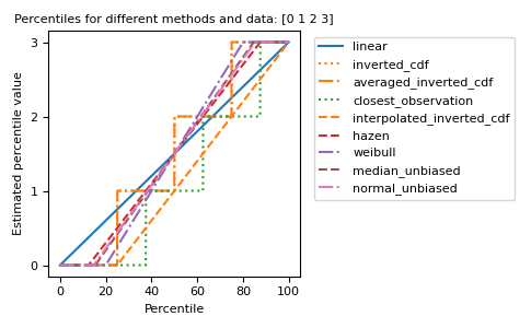
不同的方法可以圖形化地視覺化

import matplotlib.pyplot as plt

a = np.arange(4)
p = np.linspace(0, 100, 6001)
ax = plt.gca()
lines = [
    ('linear', '-', 'C0'),
    ('inverted_cdf', ':', 'C1'),
    # Almost the same as `inverted_cdf`:
    ('averaged_inverted_cdf', '-.', 'C1'),
    ('closest_observation', ':', 'C2'),
    ('interpolated_inverted_cdf', '--', 'C1'),
    ('hazen', '--', 'C3'),
    ('weibull', '-.', 'C4'),
    ('median_unbiased', '--', 'C5'),
    ('normal_unbiased', '-.', 'C6'),
    ]
for method, style, color in lines:
    ax.plot(
        p, np.percentile(a, p, method=method),
        label=method, linestyle=style, color=color)
ax.set(
    title='Percentiles for different methods and data: ' + str(a),
    xlabel='Percentile',
    ylabel='Estimated percentile value',
    yticks=a)
ax.legend(bbox_to_anchor=(1.03, 1))
plt.tight_layout()
plt.show()