numpy.histogram2d

numpy.histogram2d(x, y, bins=10, range=None, density=None, weights=None)

計算兩個資料樣本的二維直方圖。

參數:

xarray_like，形狀為 (N,)

一個包含要繪製直方圖的點的 x 座標的陣列。

yarray_like，形狀為 (N,)

一個包含要繪製直方圖的點的 y 座標的陣列。

binsint 或 array_like 或 [int, int] 或 [array, array]，可選

bin 的規格

• 如果為 int，則為兩個維度的 bin 數量 (nx=ny=bins)。

• 如果為 array_like，則為兩個維度的 bin 邊緣 (x_edges=y_edges=bins)。

• 如果為 [int, int]，則為每個維度的 bin 數量 (nx, ny = bins)。

• 如果為 [array, array]，則為每個維度的 bin 邊緣 (x_edges, y_edges = bins)。

• 組合 [int, array] 或 [array, int]，其中 int 是 bin 的數量，而 array 是 bin 邊緣。

rangearray_like，形狀為 (2,2)，可選

沿每個維度的 bin 的最左邊和最右邊邊緣（如果未在 bins 參數中明確指定）：[[xmin, xmax], [ymin, ymax]]。此範圍之外的所有值都將被視為離群值，並且不會在直方圖中計數。

densitybool，可選

如果為 False（預設值），則傳回每個 bin 中的樣本數。如果為 True，則傳回 bin 的機率密度函數，bin_count / sample_count / bin_area。

weightsarray_like，形狀為 (N,)，可選

一個值為 w_i 的陣列，用於權衡每個樣本 (x_i, y_i)。如果 density 為 True，則權重會正規化為 1。如果 density 為 False，則傳回的直方圖的值等於屬於落入每個 bin 的樣本的權重總和。

傳回值:

Hndarray，形狀為 (nx, ny)

樣本 x 和 y 的二維直方圖。x 中的值沿第一個維度繪製直方圖，而 y 中的值沿第二個維度繪製直方圖。

xedgesndarray，形狀為 (nx+1,)

沿第一個維度的 bin 邊緣。

yedgesndarray，形狀為 (ny+1,)

沿第二個維度的 bin 邊緣。

另請參閱

histogram

一維直方圖

histogramdd

多維直方圖

註解

當 density 為 True 時，傳回的直方圖是樣本密度，定義為 bin 值的總和與 bin 面積的乘積 bin_value * bin_area 為 1。

請注意，直方圖不遵循笛卡爾坐標慣例，其中 x 值在橫坐標上，而 y 值在縱坐標軸上。相反地，x 沿陣列的第一個維度（垂直）繪製直方圖，而 y 沿陣列的第二個維度（水平）繪製直方圖。這確保與 histogramdd 的相容性。

範例

>>> import numpy as np
>>> from matplotlib.image import NonUniformImage
>>> import matplotlib.pyplot as plt

建構具有可變 bin 寬度的二維直方圖。首先定義 bin 邊緣

>>> xedges = [0, 1, 3, 5]
>>> yedges = [0, 2, 3, 4, 6]

接下來，我們建立一個具有隨機 bin 內容的直方圖 H

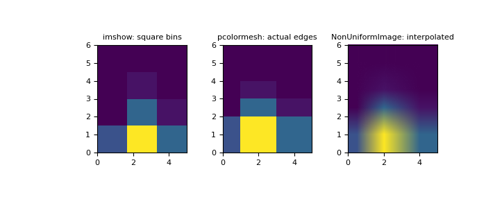
>>> x = np.random.normal(2, 1, 100)
>>> y = np.random.normal(1, 1, 100)
>>> H, xedges, yedges = np.histogram2d(x, y, bins=(xedges, yedges))
>>> # Histogram does not follow Cartesian convention (see Notes),
>>> # therefore transpose H for visualization purposes.
>>> H = H.T

imshow 只能顯示方形 bin

>>> fig = plt.figure(figsize=(7, 3))
>>> ax = fig.add_subplot(131, title='imshow: square bins')
>>> plt.imshow(H, interpolation='nearest', origin='lower',
...         extent=[xedges[0], xedges[-1], yedges[0], yedges[-1]])
<matplotlib.image.AxesImage object at 0x...>

pcolormesh 可以顯示實際邊緣

>>> ax = fig.add_subplot(132, title='pcolormesh: actual edges',
...         aspect='equal')
>>> X, Y = np.meshgrid(xedges, yedges)
>>> ax.pcolormesh(X, Y, H)
<matplotlib.collections.QuadMesh object at 0x...>

NonUniformImage 可以用於顯示具有內插的實際 bin 邊緣

>>> ax = fig.add_subplot(133, title='NonUniformImage: interpolated',
...         aspect='equal', xlim=xedges[[0, -1]], ylim=yedges[[0, -1]])
>>> im = NonUniformImage(ax, interpolation='bilinear')
>>> xcenters = (xedges[:-1] + xedges[1:]) / 2
>>> ycenters = (yedges[:-1] + yedges[1:]) / 2
>>> im.set_data(xcenters, ycenters, H)
>>> ax.add_image(im)
>>> plt.show()

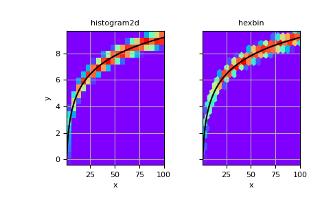
也可以建構不指定 bin 邊緣的二維直方圖

>>> # Generate non-symmetric test data
>>> n = 10000
>>> x = np.linspace(1, 100, n)
>>> y = 2*np.log(x) + np.random.rand(n) - 0.5
>>> # Compute 2d histogram. Note the order of x/y and xedges/yedges
>>> H, yedges, xedges = np.histogram2d(y, x, bins=20)

現在，我們可以使用 pcolormesh 繪製直方圖，並使用 hexbin 進行比較。

>>> # Plot histogram using pcolormesh
>>> fig, (ax1, ax2) = plt.subplots(ncols=2, sharey=True)
>>> ax1.pcolormesh(xedges, yedges, H, cmap='rainbow')
>>> ax1.plot(x, 2*np.log(x), 'k-')
>>> ax1.set_xlim(x.min(), x.max())
>>> ax1.set_ylim(y.min(), y.max())
>>> ax1.set_xlabel('x')
>>> ax1.set_ylabel('y')
>>> ax1.set_title('histogram2d')
>>> ax1.grid()

>>> # Create hexbin plot for comparison
>>> ax2.hexbin(x, y, gridsize=20, cmap='rainbow')
>>> ax2.plot(x, 2*np.log(x), 'k-')
>>> ax2.set_title('hexbin')
>>> ax2.set_xlim(x.min(), x.max())
>>> ax2.set_xlabel('x')
>>> ax2.grid()

>>> plt.show()